Fluctuation theorem for an optically trapped tracer in dense colloids. A simulation study

Fluctuation theorem for an optically trapped tracer in dense colloids. A

simulation study

Antonio M. Puertas1,a

Group of Complex Fluids Physics, Department of Applied Physics, University of Almer´ıa, 04120 Almer´ıa, Andaluc´ıa, Spain

Abstract. The work supplied by an external parabolic potential that traps one tracer in a colloidal system is studied in this work by computer simulations. The density of the bath is changed from zero up to values close to the glass transition, and the velocity varies over several decades from the linear behaviour in the low Peclet limit to the high Peclet limit. The work distributions are analyzed using the model for the isolated Brownian particle, where the friction coefficient and temperature of the medium have been fitted to reproduce the position distribution of the tracer in the trap. The overall agreement is good but not perfect. The region of negative works is studied in more detail using the predictions of the fluctuation theorem, finding good qualitative agreement with the model of the isolated Brownian particle. The present results indicate that the fluctuation theorem is of application in cases where the tracer dynamics is complex, as predicted by theoretical works.

1 Introduction

The fluctuation theorem (FT), developed in its various forms during the last two decades, has opened up and explained a new phenomenology of fundamental interest [1,2] with potential applications to diverse microscopic phenomena, particularly life [3]. In its general form, the FT states that the ratio of the probabilities of producing an entropyστ and an entropy−στ is positive and grows exponentially withστ (τ indicates the time interval where στ is mea-sured). Noteworthy, the FT allows negative increments of entropy, as far as they are small, and the macroscopic Sec-ond Law of Thermodynamics is recovered for big entropies. The FT was first demonstrated in many particle systems with deterministic dynamics, but later also in stochastic systems [4], and with more complex dynamics [5]. The entropy is produced by dissipating the work done by an external force on (part of) the system by means of a vis-cous medium. This medium is characterized by a viscos-ity and its rheological behaviour sets, from a macroscopic point of view, how the energy is dissipated. Two impor-tant cases can be identified in the study of the FT: if the fluctuations are measured from an equilibrium ensemble, the transient form of the fluctuation theorem is obtained, which setsP(στ)/P(₋στ)=exp (βστ); in contrast, if the fluctuations are measured in a (possibly far from equilib-rium) stationary state, the previous result is valid only for large integration times,τ.

In colloids, the FT has been derived in the overdamped limit, and experimentally tested in the transient regime for an isolated particle trapped in an external potential and dragged through the solvent [6,7]. On the other hand, op-tically trapped particles have been used experimentally to measure the local environment in dense quiescent systems, so called microrheology [8]. In passive microrheology the trap is held stationary [9–11], whereas in active

microrhe-a _{e-mail:[email protected]}

ology the tracer is dragged through the system [12–14]. The latter allows the measurement of microviscosities us-ing the equality between average external and frictionforces in the stationary regime, but its connection to the viscosity of the bulk system is still unclear [15,16]. The FT has been studied also in dense systems [17], in connection with plas-tic flow [18], or in other complex fluids such as a polymer melt [5]. In a system of hard spheres close to the glass tran-sition, Williams and Evans found that time required for the steady state FT to apply increases with the density up to the glass point, whereas the transient from of the FT ap-plies at all temperatures (in this case the tracer was pulled at constant force).

In this paper, we study the FT in dense colloidal sys-tems using computer simulations, from diluted syssys-tems up to a volume fraction of φ = 0.55. A particle is trapped in a harmonic potential, that moves through the system at constant speed. The velocity varies several decades, from the linear behaviour at low velocity to the linear behaviour at large ones. In a previous publication, the distributions of tracer position inside the trap were analysed using the framework developed for an isolated Brownian particle: the maximum and width of the distribution are set by the friction coefficient and temperature, respectively; i.e., the

bath is treated as a continuous medium. Upon increasing the trap speed, the effective friction coefficient shows a

plateau for low velocities, then decreases and reaches a lower plateau at high speeds, whereas the effective

temper-ature increases. Additionally, the dynamics of the tracer is affected by the high density of the bath and shows a

po-sition correlation function with a slowed decay, different

from the single particle dynamics, and reflecting the slow-ing down of the bath collective dynamics due to the steric hindrance. In the present work we study the work distribu-tion in the stadistribu-tionary state and check if the FT still applies for this system, despite the complex dynamics of the tracer. We find that using the e ffective parameters obtained from

EPJ Web of Conferences DOI: 10.1051/

C

Owned by the authors, published by EDP Sciences, 2013 ,

epjconf 201/

04001 (2013)

44

34404001

the position distributions reproduce satisfactorily the work distributions and its properties.

In the next section we give the details of the simula-tions and present the results of the tracer position distribu-tions and correlation funcdistribu-tions. In section 3, the results are presented and discussed in connection with the previous results on this system and theoretical predictions, and the concluding remarks are given in section 4.

2 Simulation details

In our simulations, the system is composed by 1000 quasi-hard particles undergoing damped Newtonian dynamics, to mimic colloidal dynamics. The equation of motion for particle jis:

mr¨j=

X

i

Fi j−γ0r˙j+fj(t)

+F_trap (1)

whereFi jis the force of particleidue to the soft-core po-tential V(ri j) = kBT(r/σi j)−36, withkBT the thermal en-ergy andσi j the center to center distance,γ0 is the fric-tion coefficient of the solvent and fj is a random force obeying the fluctuation dissipation theorem,hfi(t)fj(t′)i = 6kBTγ0δ(t−t′)δi j. The trap is felt only by one particle, and is introduced via a linear force:Ftrap =−k

r₋rtrap

, wherertrapis the trap minimum. Polydispersity is included to avoid crystallization at high density – a flat distribution of radii [0.9a,1.1a] withathe average particle radius. All particles have the same mass,m. In the units of the system, a=1,k_BT =1 andm=1, the friction coefficient is set to

γ0=50, and the spring constantk=1000.

In an equilibrated system, a particle is selected ran-domly and trapped in the external harmonic potential, with

rtrap moving at constant velocityvtrapalong the x-axis of the simulation box. To improve the statistics, the box is elongated along the dragging direction to dimensionsLx,L,L, withLx = 8L. The particle is dragged for a distance Lx, whereas the rest of particles undergo Brownian motion (Eq. 1 withoutFtrap). Density is reported as volume fraction, φ = 4₃πa3[1+(δ/a)2]n_c, with n_c the particle concentra-tion andδ the half-width of the radius distribution. The equations of motion were integrated using Heun’s algo-rithm[19] with a time stepδt = 5_·10−4. The position of

the tracer with respect to the trap minimum is recorded for times up tot=25000, after a lag timea/v_trap, to assure sta-tionarity. The use of damped Newtonian dynamics allows both momentum transfer to other particles and dissipation of energy to the fluid, in contrast to Newtonian dynamics or pure Brownian dynamics.

The analysis of the stationary tracer position distribu-tion in the trap was performed previously [14] using the model for an isolated Brownian particle [20]. For this model, this distribution is given by

p(α) = r

k 2πk_BT exp

n

−kα2/2kBTo (2)

whereαisx₋xst,yorz, withxstthe solution of the sta-tionary state equation, i.e. γ0vtrap = −k(xst −xtrap). For finite density,γandT must be fitted to reproduce the ob-served distribution, which indeed is Gaussian and is well modelled by the expression above with a suitable choice

10

10

10

γ

/ γ

φ = 0

φ = 0.10

φ = 0.30

φ = 0.40

φ = 0.50

φ = 0.55

10

10

10

10

10

v

10

10

T

Fig. 1.Effective friction coefficient (upper panel) and effective

temperature (lower panel) as a function of the trap velocity, as obtained from the analysis of the tracer position distributions, for different volume fractions, as labeled.

of these parameters [14]. The results of the fitting param-eters,γe f f andTe f f, are presented in Fig. 1. The effective friction coefficient shows a high plateau at low velocities

and a lower one at largervtrap, whereas the effective tem-perature goes to the bath temtem-perature in the low velocity limit and raises for larger ones. These results can be ra-tionalized considering that the energy input is dissipated in the friction with the solvent, controlled byγ0. For large ve-locities, the energy is injected in the system at a high rate, larger than the dissipation, resulting in a region around the tracer with increased mobility, i.e. larger local temperature. This is confirmed by studying the tracer position cor-relation function, which measures how fluctuations of the tracer position relax to its equilibrium value. For an iso-lated Brownian particle, this correlation function reads for thex-coordinate:

hx˜(t+τ) ˜x(t)_i=kBT

k exp (−kτ/γ0)+

vtrapγ_k0

2

. (3)

where ˜x=x₋xtrap. This is presented in Fig. 2 for different densities at constant trap speed. Upon increasing the den-sity, the correlation function shows a clear deviation from the single exponential decay, in connection with the diff

10-2 10-1 100 101

t

-0.5 0.0 0.5 1.0 1.5 2.0 2.5

k ( <x(t)x(0)> - x

st

2

)

φ = 0.50 φ = 0.40 φ = 0.20

Single particle

v

= 1

Fig. 2.Tracer position correlation functions for different

densi-ties, as labeled, at a constant trap velocityvtrap=1. Note that the long time plateau is substracted in all cases, to allow comparison of the different states.

the global decay to longer times (due to the increase of the friction coefficient).

3 Results and discussion

The work done on the particle by the trap during a time intervalτ,Wτ, is then dissipated by the medium or trans-ferred to other particles, and ultimately dissipated. For an isolated particle in a medium with friction and neglecting the inertial term, this work is Gaussian distributed, and in the stationary state reads [21,22]:

P_S(Wτ) = exp n

−[Wτ−MS(τ)]2/2VS(τ)

o

√₂ πVS(τ)

(4)

whereMS(τ) =γ0v2trapτis the average work, andVS(τ)= 2γ0kBTv2trap

τ₋τ_rh1₋e−τ/τri, with_τ

r=γ0/k[21,22]. In this model, this work is dissipated to the medium directly. This expression correctly reproduces the work distribution of the isolated particle in the simulations, as shown below.

In the simulations,Wτis calculated as:

Wτ=

Z τ

0 dtvtrapFtrap, (5)

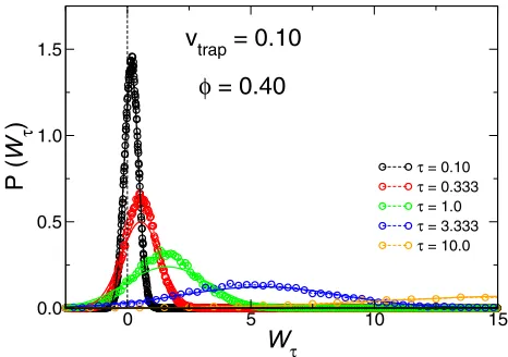
The effect of the time interval is presented in Fig. 3, where

the distributions for φ = 0.40 and vtrap = 0.1 are pre-sented for different values ofτ. Note that the average work is always positive, but the distributions extend to nega-tive values of the work, indicating that the particle does

work on the trap, i.e. the particle is pulling the trap. As

expected, this tail disappears for large τ, recovering the macroscopic form of the Second Law of Thermodynam-ics. All the distributions are Gaussian, as predicted by the single particle model, Eq. 4, and are qualitatively repro-duced by the model if the solvent parameters (friction co-efficient and temperature) are substituted by the effective

parameters obtained from the analysis of the steady tracer position distributions.

The work distributions for different densities and

ve-locities are presented in Fig. 4, and compared with the

0 5 10 15

W

0.0 0.5 1.0 1.5

P (

W

)

τ = 0.10

τ = 0.333

τ = 1.0

τ = 3.333

τ = 10.0

v

= 0.10

φ

= 0.40

Fig. 3. Distribution of work done by the trap on the particle for

vtrap=0.10 andφ=0.40 and different time intervals, as labeled. The circles are data from simulations and the lines predictions from eq. 4.

theoretical calculations. As mentioned above, the distribu-tions are Gaussian, except at low density and high veloc-ity (see the red points in the lower panel). Upon increas-ing the density (at constant trap velocity), more work is dissipated to the medium, because its effective viscosity is

higher, and the distribution is wider since the temperature is also higher. For faster velocities, much larger works are done by the trap, increasing asv2_trap, although the friction coefficient decreases. In this limit, the work is only

pos-itive, approaching the macroscopic Second Law of Ther-modynamics. The solid lines represent the calculated work distribution with expression 4 using the effective

parame-ters from the position distributions. The overall agreement between the calculated distributions and simulation results is good but not perfect (note that all parameters in Eq. 4 are fixed), particularly the maximum is very well reproduced, except at small density and large velocities. It is important to note that although two mechanisms are possible to dissi-pate the work (namely, friction of the tracer and collisions with other particles), these merge giving a Gaussian distri-bution with a single maximum. Only in the case of large velocities and low density the two mechanisms can be re-solved, showing a distribution that deviates clearly from the Gaussian behaviour (red points in the lower panel).

The FT can be further tested in the region of small and negative works by checking the following property in the stationary state:

P_S(Wτ)

PS(−Wτ) = exp

( _βW

τ 1−ǫ(τ)

)

(6)

whereǫ(τ)=τr

h

1−e−τ/τri_/τ[21,22]. As the time interval

τdivergesǫ(τ_{→ ∞})_→0, and the above expression tends to the more conventional form of the FT:P_S(Wτ)/P_S(₋Wτ)_→ eβWτ(_{τ→ ∞}). The latter is valid for all_τin the transient

regime and has been experimentally tested for a single col-loidal particle trapped in a harmonic potential [6,7]. The FT in the stationary state is tested in Fig. 5 for the same state as in Fig. 3. As predicted, ln(P_S(Wτ)/P_S(₋Wτ)) is indeed proportional to Wτ, and the slope decreases with increasing integration times, and approaches 1 for largeτ. In Fig. 6 the test of the FT is presented for different

-1 0 1 2 3 0.0

0.2 0.4 0.6 0.8 1.0

P (

W

)

0 20 40 60 80

0.00 0.02 0.04 0.06 0.08

P (

W

)

φ = 0.

φ = 0.10

φ = 0.30

φ = 0.50

φ = 0.55

1000 2000 3000 4000

W

0.002 0.004 0.006 0.008

P (

W

)

v

= 0.10

v

= 1.0

v

= 10

Fig. 4. Distribution of work done by the trap on the particle for

vtrap =0.10,1.0 and 10 from top to bottom. Different densities are presented – note the di fferentx-scale in the three panels. The circles are data from simulations and the lines predictions from eq. 4 with the effective parameters from the position distributions.

-2 -1 0 1 2

W

-4.0 -2.0 0.0 2.0 4.0

ln (P (

W

) / P

(-W

))

τ = 0.10

τ = 0.333

τ = 1.0

τ = 3.333

τ = 10.0

v

= 0.10

φ

= 0.40

Fig. 5. Test of the FT forvtrap =0.10 andφ=0.40 and

differ-ent time intervals, as labeled. The thick black line represdiffer-ent the expected long time behaviour, slope 1.

-2

-1

0

1

2

-4.0 -2.0 0.0 2.0 4.0

ln (P (

W

)/P

(-W

))

φ = 0

φ = 0.10

φ = 0.30

φ = 0.50

φ = 0.55

-7.5 -5 -2.5 0 2.5 5 7.5

W

-7.5 -5.0 -2.5 0.0 2.5 5.0 7.5

ln (P (

W

)/P

(-W

))

v

= 0.10

v

= 1.0

Fig. 6. Test of the FT forvtrap =0.10 (upper panel) andvtrap =

1.0 (lower panel) and different volume fractions, as labeled. The thick black lines have slope 1.

v=1.0 (lower panel). For the smaller velocity, the slope of the data increases with the volume fraction, starting from slope 1 for the dilute system, whereas for the larger veloc-ity all the data almost collapse onto the same curve, with a slope close to 1. These findings can be rationalized with the single-particle model as follows: becauseτr = γ/k, upon increasing the volume fraction of particles, τr increases and so doesǫ(τ) at constantτ; the prefactor 1/(1₋ǫ(τ)) thus increases in eq. 6, as observed in Fig. 6. For the larger velocity, the friction coefficient is smaller (see Fig. 1), and

ǫ(τ) is close to zero for thisτ.

These results are in agreement with other simulation studies [17] where a constant force is applied to the tracer instead of the parabolic trap used here. In both cases, upon approaching the glass transition, i.e. slowing down the sys-tem dynamics,ln(PS(Wτ)/PS(−Wτ)) deviates fromWτ, con-firming the expectations of the single particle approxima-tion. On the theoretical side, Toyabe and Sano [5] corrob-orated that the FT can be formulated using the generalized Langevin equation, where the friction with the solvent con-tains a memory term, establishing a link with dense sys-tems close to the glass transition.

4 Conclusions

Brownian particle, i.e. treating the colloidal bath as con-tinuous medium. The distribution of the tracer position in the trap was previously analyzed with the same model, and it was found that the friction coefficient and temperature

rameters, the work distributions have been calculated and compared with the simulation results, finding good agree-ment, particularly in the position of the maximum work. The agreement is worse in the case of the width of the dis-tribution, but the overall trends are correctly captured. The fluctuation theorem is further tested by studying the ratio of positive to negative works, finding also that the expec-tations from the theory are fulfilled.

The present results give more evidence supporting that the fluctuation theorem can be applied to complex systems with non-simple dynamics with semi-quantitative agree-ment. In the present system, the particle dynamics shows a two-step decay due to the complex dynamics of the bath, approaching the glass transition. The dissipation of work is therefore performed via two routes: by direct friction with the solvent, and by collisions with other particles and their friction with the solvent, the latter being absent in the the-oretical models used.

References

1. D.J. Evans, E.G.D. Cohen, G.P. Morriss, Phys. Rev. Lett.712401 (1993).

2. D.J. Evans, D.J. Searles, Adv. Phys.51, (2002) 15929. 3. C. Bustamante, J. Liphardt, F. Ritort, Phys. Today58,

(2005) 43.

4. J.L. Lebowitz, H. Spohn, J. Stat. Phys.95, (1999) 333. 5. S. Toyabe, M. Sano, Phys. Rev. E77, (2008) 041403. 6. G.M. Wang, E.M. Sevick, E. Mittag, D.J. Searles, D.J.

Evans, Phys. Rev. Lett.89, (2002) 050601.

7. D.M. Carberry et al. Phys. Rev. Lett.92, (2004) 140601. 8. P. Cicuta, A.M. Donald, Soft Matter3, (2007) 1449. 9. N. Greinert, T. Wood, P. Bartlett, Phys. Rev. Lett.97,

(2006) 265702.

10. B. Luki´c, S. Jeney, Z. Sviben, A. J. Kulik, E.-L- Florin, and L. Forr´o,Phys. Rev. E,76, 011112 (2007).

11. A.M. Puertas, AIP Proceedings1319, (2010) 141. 12. A. Meyer, A. Marshall, B.G. Bush, E.M. Furst, J.

Rheol.50, (2006) 77.

13. I. Sriram, A. Meyer and E.M. Furst, Phys. Fluids22, 062003 (2010).

14. L.G. Wilson, A.W. Harrison, W.C.K. Poon, A.M. Puertas. Europhys. Letters93, (2011) 58007.

15. T.M. Squires, J.F. Brady, Phys. Fluids 17, (2005) 073101.

16. T.M. Squires, Langmuir24, (2008) 1147.

17. S.R. Williams, D.J. Evans, Phys. Rev. Lett.96, (2006) 015701.

18. J.A. Drocco, C.J. Olson Reichhardt, C. Reichhardt, Eur. Phys. J. E34, (2011) 117.

19. W. Paul, D.Y. Yoon, Phys. Rev. E52, (1995) 2076. 20. R.D. Astumian, J. Chem. Phys.126, (2007) 111102. 21. O. Mazonka, C. Jarzynski, e-print cond-mat/9912121

(1999).

22. R. van Zon, E.G.D. Cohen, Phys. Rev. E67, 046102 (2003).