Chasing Shadows in the Outer Solar System

(1)

University of Pennsylvania

ScholarlyCommons

Publicly Accessible Penn Dissertations

Spring 5-17-2010

Chasing Shadows in the Outer Solar System

Federica Bianco

University of Pennsylvania, [email protected]

Follow this and additional works at:http://repository.upenn.edu/edissertations

Part of theInstrumentation Commons, and theThe Sun and the Solar System Commons

This paper is posted at ScholarlyCommons.http://repository.upenn.edu/edissertations/176

For more information, please [email protected].

Recommended Citation

Bianco, Federica, "Chasing Shadows in the Outer Solar System" (2010).Publicly Accessible Penn Dissertations. 176.

(2)

Chasing Shadows in the Outer Solar System

Abstract

The characteristics of the populations of objects that inhabit the outer solar system carry the fingerprint of the processes that governed the formation and evolution of the solar system. Occultation surveys push the limit of observation into the very small and distant outer solar system objects, allowing us to set constraints on the structure of the Kuiper belt, Scattered disk and Sedna populations. I collected, reduced, and analyzed vast datasets looking for occultations of stars by outer solar system objects, both working with the Taiwanese American Occultation Survey (TAOS) collaboration and leading the MMT/Megacam occultation effort. Having found no such events in my data, I was able to place upper limits on the Kuiper belt, scattered disk and Sedna population. These limits and their derivation are described here.

Degree Type

Dissertation

Degree Name

Doctor of Philosophy (PhD)

Graduate Group

Physics & Astronomy

First Advisor

Charles R. Alcock

Second Advisor

Pavlos Protopapas

Third Advisor

Matthew Lehner

Keywords

Solar System, Kuiper Belt, Sedna, Occultations, Fresnel Diffraction, Fast Photometry

Subject Categories

(3)

CHASING SHADOWS IN THE OUTER SOLAR SYSTEM

Federica Bianco

A DISSERTATION

in

Physics and Astronomy

Presented to the Faculties of the University of Pennsylvania

in Partial Fulfillment of the Requirements for the degree of Doctor of Philosophy

2010

Charles R. Alcock

Supervisor of Dissertation

Ravi Sheth

(4)

Acknowledgments

I ain’t no physicsist, but i know what matters!

Popeye

The work presented in Chapers 3, 4 & 5 was accomplished with the

col-laboration of the entire TAOS team: C. Alcock (Harvard-Smithsonian Center for

Astrophysics), T. Axelrod (Steward Observatory), Y.-I. Byun (Department of

As-tronomy, Yonsei University), W. P. Chen (Institute of AsAs-tronomy, National

Cen-tral University, Taiwan), N. K. Coehlo (Department of Statistics, University of

California Berkeley), K. H. Cook (Institute for Geophysics and Planetary Physics,

Lawrence Livermore National Laboratory), R. Dave (Initiative in Innovative

Com-puting at Harvard), I. de Pater (Department of Astronomy, University of

Cali-fornia Berkeley), J. Giammarco (Department of Astronomy and Physics,

East-ern University; Department of Physics, Villanova University), D.-W. Kim

(De-partment of Astronomy, Yonsei University), S.-K. King (Institute of Astronomy

and Astrophysics, Academia Sinica), T. Lee (Institute of Astronomy and

Astro-physics, Academia Sinica), M. J. Lehner (Institute of Astronomy and AstroAstro-physics,

Academia Sinica; Department of Physics and Astronomy, University of

Pennsylva-nia; Harvard-Smithsonian Center for Astrophysics), H.-C. Lin (Institute of

Astron-omy and Astrophysics, Academia Sinica), J. J. Lissauer (Space Science and

(5)

Particle Astrophysics and Cosmology), S. Mondal (Aryabhatta Research Institute

of Observational Sciences), P. Protopapas (Initiative in Innovative Computing at

Harvard), J. A. Rice (Department of Statistics, University of California Berkeley),

M. E. Schwamb (ivision of Geological and Planetary Sciences, California Institute

of Technology), J.-H. Wang (Institute of Astronomy and Astrophysics, Academia

Sinica; Institute of Astronomy, National Central University, Taiwan), S.-Y. Wang

(Institute of Astronomy and Astrophysics, Academia Sinica), C.-Y. Wen(Institute

of Astronomy and Astrophysics, Academia Sinica), and Z.-W. Zhang (Institute of

Astronomy, National Central University, Taiwan),

This work was supported in part by the NSF under grant AST-0501681

and by NASA under grant NNG04G113G to Harvard University. Observations

re-ported in Chapter 2 were obtained at the MMT Observatory, a joint facility of

the Smithsonian Institution and the University of Arizona. Work at National

Cen-tral University was supported by the grant NSC 96-2112-M-008-024-MY3. Work at

Academia Sinica Institute of Astronomy & Astrophysics was supported in part by

the thematic research program AS-88-TP-A02. Work at Yonsei University was

sup-ported by Korea Astronomy and Space Science Institute. The work of N. Coehlo

was supported in part by NSF grant DMS-0636667 to the University of

Califor-nia Berkeley. Work at Lawrence Livermore National Laboratory was performed in

part under USDOE Contract W-7405-Eng-48 and Contract DE-AC52-07NA27344.

Work at SLAC was performed under USDOE contract DE-AC02-76SF00515. Work

at NASA Ames was supported by NASA’s Planetary Geology & Geophysics

Pro-gram. This research has made use of SAOImage DS9, developed by Smithsonian

Astrophysical Observatory.

As for the rest:

(6)

molte cose da dire e fare che ci scoraggiamo e non diciamo o facciamo mai. vi voglio

bene e mi mancate. e vi sono grata per tutte le opportunit`a che mi avete dato.

momdadhobogregberngeorge, thanks for being patient.

greg again, for covering up for me, walking the dog for me, making phone calls for

me, cleaning up for me, driving around for me... and keeping irony going, most of

the times. i could have not done this – or much of anything else really – without

you.

Of course Charles, for finding the time, despite the many many more things that

should have come ahead of my questions and doubts, family, government, telescope

building. I know you lost many hours of sleep. And for the support in times of

crisis, of which there were many, such as when almost got deported.

Pavlos, a very tolerant man. special thanks for keeping me calm at times and keeping

me creative at others.

Matt, for escorting me in many Taiwan trips, helping me ordering the right liquor in

Chinese, facilitating intercultural communication, teaching me that fewer is better,

when it comes to lines of code, and wanting to have as little as possible to do with

my fits: it worked to control them.

Working on this thesis gave me the great opportunity to travel to Asia

(7)

ABSTRACT

CHASING SHADOWS IN THE OUTER SOLAR SYSTEM

Federica Bianco

Charles R. Alcock

The characteristics of the populations of objects that inhabit the outer

solar system carry the fingerprint of the processes that governed the formation and

evolution of the solar system. Occultation surveys push the limit of observation into the very small and distant outer solar system objects, allowing us to set

con-straints on the structure of the Kuiper belt, Scattered disk and Sedna populations.

I collected, reduced, and analyzed vast datasets looking for occultations of stars by outer solar system objects, both working with the Taiwanese American Occultation

Survey (TAOS) collaboration and leading the MMT/Megacam occultation effort.

Having found no such events in my data, I was able to place upper limits on the Kuiper belt, scattered disk and Sedna population. These limits and their derivation

(8)

List of Tables

2.1 MMT/Megacam survey observed fields . . . 27

2.2 MMT/Megacam survey data set parameters. . . 28

3.1 TAOS dataset parameters (3–telescope data) . . . 55

3.2 Distribution of synthetic events . . . 72

(11)

List of Figures

1.1 Outer Solar System taxonomy . . . 6

1.2 TNO discoveries by year and R magnitude . . . 8

1.3 Luminosity distribution of KBOs from Fuentes & Holman (2008) . . . 9

1.4 Occultation geometry . . . 11

1.5 Diffraction by a TNO ocultation . . . 13

1.6 Diameter – semimajor-axis phase space detectability . . . 15

2.1 Simulated diffraction pattern for an MMT/Megacam hypothetical target . . . 21

2.2 Megacam focal plane . . . 22

2.3 Images generated by conventional camera use and by continuous– readout . . . 24

2.4 Frequency analysis of MMT/Megacam continuous–readout data . . . 26

2.5 Image motion and PSF width fluctuation for our continuous–readout data . . . 31

2.6 MMT/Megacam continuous–readout lightcurves before and after de-trending . . . 34

2.7 Implantation of occultation signatures in our data . . . 35

2.8 Non-parallel, simultaneous CCD motion features . . . 39

2.9 Detection efficiency and number of false positives . . . 40

2.10 Detection efficiency and effective solid angle of our survey . . . 45

2.11 Duration and flux drop caused by occultations in the size and distance regime we are considering . . . 47

2.12 Upper limits to the surface density of KBOs from the MMT/Megacam occultation survey . . . 48

3.1 Distribution of magnitudes and SNR for the TAOS target stars . . . 55

3.2 SNR versus TAOS instrumental magnitude . . . 56

3.3 Distribution of angles from opposition for the TAOS targets . . . 56

3.4 Diffraction table and synthetic diffraction features . . . 65

3.5 Steps of the generation of a simulated occultation event . . . 68

(12)

3.7 Implanted occultations recovered by our pipeline . . . 73 3.8 Our recovery efficiency for 3 km KBOs as a function of observational

parameters . . . 76

4.1 Effective solid angle of our survey . . . 79 4.2 Model independent upper limits to the surface density of KBOs from

the TAOS survey . . . 80 4.3 PS05 model and expected event rate for TAOS . . . 85 4.4 Modeling of the KB04 results: theD = 0.5₋30 km region. . . 86 4.5 KB04 model and expected event rate for TAOS with excess centered

at 5.5 km . . . 91 4.6 KB04 model and expected event rate for TAOS with excess centered

at 1.6 km . . . 92 4.7 BCB09 model and expected event rate for TAOS . . . 93 4.8 Generic three–slopes parametric modeling of the KBO size

distribu-tion and constraints from the TAOS survey . . . 93

5.1 Occultation signatures of aD= 10 km and a D = 5 km objects at 400 AU and their detectability . . . 100 5.2 Minimum coverage of our survey . . . 102 5.3 Maximum number density of D _≥ 1 km objects allowed by our

(13)

Chapter 1 Introduction

1.1 Historical note

It could be argued that interest in the solar system initiated scientific

thinking. All ancient cultures that left a written or graphical record left some

rep-resentation of the Sun and the Moon, of the planets and the fixed stars. Dynamical

theories of what was then thought of as the entire Universe are among the first

records of most cultures. Early Americans, Greeks, Egyptians, Chinese,

Babylo-nians, Indian, Celtic, and Islamic cultures, all generated cosmological theories to

describe and explain the rising and setting of the sun, the phases of the moon, the

motions of the planets across the sky, the immobile stars and the changing of

sea-sons. The motions of solar system objects, which we now call ephemerides, were

studied well enough by the ancient Egyptians that they were able to build enormous

tomb structures that allow the Sun to shine in precisely once a year and only once

a year. Mechanical tools (e.g.: the Antikythera) were designed to simplify the

cal-culation of an ephemeris, and are considered today to be precursors to the modern

(14)

Ancient Greek philosophers payed great attention to astronomy, and

pro-duced a variety of theories to describe the motion of objects in the sky, including

some early heliocentric theories (Aristarchus of Samos, Batten 1981), untill the

Aris-totelian idea of concentric spheres prevailed and dominated in some form or another,

until Copernicus and Galileo1_{. Galileo, Kepler, Newton, and later Kant, started}

in-vestigating the forces which keep planets moving in their orbits, what holds them

up in place and puts them in motion.

Remarkably, after over 2000 years of solar system science, we have probed

only as little as 10−9 _{of the space occupied by the solar system: the inner portion,}

which contains over 99% of its mass. The outskirts of the solar system are however

still unexplored. Outside of the orbit of Neptune the solar system is populated

by small (thousands of kilometers down to dust grain size) icy bodies, arranged in

different structures: the Kuiper belt, the Oort cloud, and the scattered disk. Our

direct observational knowledge is limited to relatively large objects populating the

Kuiper belt and the scattered disk.

1.2 Formation

In the current solar system formation and evolution scenario planets formed

by gravitational instabilities in the protoplanetary nebula: a disk of gas and dust

surrounding the Sun.

Throughout the remainder of this section I will refer to the solar system

evolution model that came to be known as the Nice model (Gomes et al., 2005a;

Morbidelli et al., 2005; Tsiganis et al., 2005; Levison et al., 2008, and references

therein), one of the most successful scenarios to explain the current configuration of

1

(15)

solar system objects. In this model the four giant planets, Jupiter, Saturn, Uranus,

and Neptune, originally formed from the circumsolar disk of dust and gas on nearly

circular orbits between 5 and 17 AU, a much more compact configuration than that

which we see now. Gravitational instabilities in the disk caused accretion processes

to form large planets out of the dust and small planetesimals inhabiting the disk.

Outside of the planetary orbits there remained a disk of icy planetesimals, extending

out to _∼35 AU.

In the early chaotic solar system the planetesimals which were residing

within the planetary orbits suffered occasional gravitational encounters with the

outermost giant planets, which changed the planetesimal orbits, initially scattering

them inward. In turn, the outermost giant planets began migrating outward to

preserve angular momentum. As they were pushed into the inner regions of the solar

system, the planetesimals began to interact with Jupiter, which on account of its

much larger mass dramatically affected their orbital parameters at each encounter.

The icy bodies that encounter Jupiter were sent onto highly elliptical orbits or

ejected altogether from the solar system, and to compensate for the loss of angular

momentum Jupiter migrated inward.

After several hundred million years Jupiter and Saturn crossed their 1:2

mean motion resonance and that suddenly increased their orbital eccentricities,

destabilizing the entire solar system. Uranus’s and Neptune’s eccentricities were

increased as a result of the interaction with Saturn, and as they migrated outward

they pushed planetesimals outward as well, wiping the region which they transited

clean of icy bodies. Through these interactions, the orbits of Uranus and Neptune

were again circularized. Meanwhile the vast majority of planetesimals were shuffled

and over 90% of the original planetesimals mass was removed.

(16)

Neptune, a large portion remained in low inclination orbits, and some of them got

captured in mean motion resonances with Neptune. These formed the Kuiper belt,

first predicted by Kenneth Edgeworth in 1943, and later by Gerard Kuiper in 1951.

The Kuiper belt is a flat structure, extending from the orbit of Neptune (_∼30 AU)

out to about 50 AU, where observations reveal an outer edge (Jewitt et al., 1998).

A fraction of the Kuiper belt planetesimals were excited, possibly through

resonance and weak chaos associated to secular Kozai mechanisms (Volk & Malhotra,

2009), and their inclination distribution increased, forming the scattered disk and

extended scattered disk. The scattered disk is a family of TNOs populated by

objects with perihelia q > 30 AU and with inclinations as high as i _∼ 40◦_{. The}

extended scattered disk is a population of object whose perihelia is large enough to

be decoupled from Neptune (see Figure 1.1).

Many planetesimals bounced in and out of the inner solar system by

re-peated encounters with Jupiter. These interactions increased the eccentricities e

of their orbits. The planetesimals that were not ejected via this mechanism were

hand off out to Neptune. Interactions with Neptune continued increasing the

or-bital sami-major axis while preserving the perihelion distance of these planetesimals.

Once their orbits reached _∼3,000 AU the influence of the mean gravitational field

of the Galaxy became important, and their perihelia lifted from the region of

influ-ence of Neptune. The inclination distribution of planetesimals in orbit farther than

3,000 AU increased dramatically: these planetesimals formed the Oort cloud, an

isotropic structure of icy bodies which might extend farther out than 105 _AU

(Dun-can et al., 1987).

The existence of a cloud of icy bodies in the out skirts of the solar system

was originally proposed by J. Oort in 1950 (Oort, 1950), in order to explain the long

(17)

their perihelion passage and they provide the only observational evidence we have

of the Oort cloud.

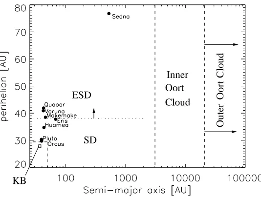
Figure 1.1 shows a schematic partition of the perihelion and semi-major

axis phase space and the TNO families that occupy it. The classical Kuiper belt

(KB) lies on the bottom left corner of the plot. An empty square shows the position

of the median perihelion and semi-major axis of the classical and resonant KBOs.

At q > 30 AU and a > 50 AU lays the scattered disk (SD). The extended

scattered disk comprises objects with perihelia larger than q _∼ 38 AU, which are

decoupled from Neptune. The inner Oort cloud start outward of a = 3,000 AU

and the outer Oort cloud at a > 20,000AU. The reader is cautioned that this

schematic separation in q₋a space is only for reference. Other families are here

ignored, such as the resonant populations, Plutinos, and Centaurs. Furthermore,

the TNO taxonomy is not unique, and TNO nomenclature is often based on other

variable, q₋e, q₋i, color, etc. (Barucci et al., 2005; Gladman et al., 2008, and

references therein)

The Nice model model is able to explain many features of our solar system:

it reproduces the current planetary orbits, the existence of objects in the Kuiper

belt and in resonance with Neptune, the asteroid belt, as a relic of the planetary

nebula not affected by the migration of Uranus and Neptune. It is however unable

to explain the existence of an outer edge in the Kuiper belt, it predicts more mass to

be left in the solar system than we know of, and itcannot explain the the existence

of Sedna.

Sedna was discovered in 2004 (Brown et al., 2004). None of the formation

mechanisms in the literature at the time of discovery were able to place orbits in this

region of the perihelion and semi-major axis phase space: this region is inaccessible

(18)

ESD

KB

Outer

Cloud

Oort

Cloud Oort

Inner

SD

Figure 1.1: Schematic partition of the perihelion and semi-major axis phase space. Five distinct dynamical families are identified: the Kuiper belt (KB) in the bottom left corner, the scattered disk (SD), the extended scattered disk (ESD), the inner and outer Oort cloud. The largest observed TNOs are shown (black circles), as well as the median values

of q and aof the Kuiper belt (open square).

the inner solar system. To date no surveys have detected any other object in orbit

similar to Sedna, and its existence is still unexplained in the current formation and

evolution scenarios without invoking the presence of a perturbation from an external

body (see Section 5).

1.3 Observational techniques to explore the outer

solar system

Populated by small and cold bodies the outer solar system is among the

most challenging observational targets in astrophysics today. Direct detection of

Trans Neptunian Objects (TNOs) is a difficult task. These objects typically range

(19)

are seen in reflected Sun light, thus getting fainter as_∼∆4_{, where ∆ is the distance}

to the Earth. Furthermore, they move across the sky at a rate of _∼3 arcsec/hour,

making it impossible to increase their detectability just by increasing the integration

time, and rendering any technique used to increase the depth of a survey, such as

stacking, much harder to perform.

The very first Kuiper belt object to be observed was Pluto (134340 Pluto),

discovered in 1930 by Clyde Tombaugh. Pluto has a mean magnitude R _∼ 14,

and a diameter of about 2,390 km. For its size, Pluto is exceptionally bright due

to a high albedo of about 50%. Classified as a planet until 2006, Pluto is today

the second largest known KBO after Eris (136199 Eris), which has a diameter of

about 2,500 km and an apparent magnitude of R _∼ 18.4. Eris was discovered in

2005 (Brown et al., 2005).

Over 30 years passed between the first detection of Pluto and the discovery

of the next KBO. Jewitt and Luu announced the “Discovery of the candidate Kuiper

belt object” in a Nature paper on August 30th 1992, the object known as 15760

1992 QB1. Six months later they reported a second object in the Kuiper belt

region, 181708 1993 FW. Today (March 2, 2010) 1099 observed TNOs are cataloged

by the Minor Planet Center2_{, which keeps track of all TNOs and minor planet}

observations and creates ephemerides to predict their position in time. The rate of

TNO discoveries, however, peaked in 2001 and it has been decreasing ever since (see

Figure 1.2, left).

To date all observed TNOs are brighter than R > 30. Figure 1.2, right,

shows the R-magnitude distribution of known KBOs. The majority of the observed

objects are in the magnitude range 23_≤R _≤26; the median magnitude of observed

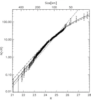
TNOs is _hR_{i ∼} 23.5. Figure 1.3, from Fuentes & Holman (2008), shows the

2

(20)

0 20 40 60 80 100 120 140 160 180

1992 1994 1996 1998 2000 2002 2004 2006 2008

number of discovered TNOs

year

16 18 20 22 24 26 28 0 50 100 150 200 250 300 350 400 450 R

Figure 1.2: Left: number of discovered TNOs per year. Right: number of observed

TNOs as a function ofRmagnitude. The vast majority of observed TNOs have apparent

magnitude in the range 22_≤R_≤26. Brighter KBOs are rare and fainter KBOs, although

more numerous, are hard to detect

cumulative size distribution of KBOs as a function of R magnitude. Most observed

KBO are individually plotted. The density of observed KBOs with 23 _≤ R _≤ 26

allows a firm determination of the size distribution in this magnitude range (see

Section 1.4). Only three objects have been observed that are fainter than magnitude

R = 26.5: R = 26.7, 28.0 and 28.2, corresponding to diameters of respectively 44,

28 and 25 km assuming, as customary, an albedo of 4% (Bernstein et al., 2004).

Future all sky surveys such as Pan–STARRS3 _{and LSST}4 _{will discover}

many more R <26 objects (Jewitt, 2003), and data mining projects are in progress

to detect faint targets in archival HST data (Fuentes et al., 2009a). The

observa-tional barrier at R_∼30 is however hard to overcome.

1.3.1 Diffraction dominated occultations of bright stars

Bailey (1976) proposed that small TNOs could be seen indirectly at their

passage across the line of sight to a star. This event, today known as anoccultation,

would produce a variation in the flux of the observed star which in principle can

3

http://pan-starrs.ifa.hawaii.edu/public/science-goals/solar-system.html

4

(21)

(22)

be observed, much like in planetary transit surveys. The dramatic difference from

planetary transit surveys is however in the geometry of the system: in this technique

a distant star, often an unresolved point source, is occulted by a near-by object

with a finite angular size. Noticeably, for the events of interest, the geometry of

the system is such that occultations by outer solar system objects too small to be

observed directly are typically diffraction dominated events.

If we consider a roughly kilometer size object in the Kuiper belt (30-50 AU)

we have the case of a light wave obstructed by an object at finite distance, where

the diffractor size is large compared to the wavelength. In this regime diffraction is

properly described in terms of the Huygens–Fresnel principle. The discussion that

follows is based on Born & Wolf (1980) and on Roques et al. (1987).

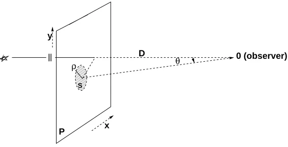
Modeling the occulting object as a flat opaque screen S, and neglecting

the scattering of light at the edges of the occulter, the diffraction amplitude aS of a

monochromatic plane wave at wavelength λ can be derived at the observing point

0 by the Fresnel–Kirckoff diffraction formula as follows: assume the occulter S lays

on a plane P perpendicular to the line of sight, at a distance D from the observer

(and infinitely far from the source of light in the plane wave approximation), then

aS(0) = N

Z Z

P−S

e(2iπλ

√

X2₊_Y2₊_D2₋_D)

√

X2₊_Y2 ₊_D2 (1 + cosθ) dXdY, (1.1)

where P ₋S is the plane of the occulting screen, θ the angular distance from the

center of the diffractor, and X and Y the Cartesian distance from the center of

the screen S and the point perpendicular to the line of sight on the plane P (see

Figure 1.4). This intensity is normalized to aS(0) = 1 away from the objects by

(23)

000 000 000 000 000 000 000 000 111 111 111 111 111 111 111 111 S P x y

D _{0 (observer)}

ρ θ

Figure 1.4: Schematic representation of an occultation. The occulter S is modeled as a

circular disk laying on the planeP. The occultation is observed by an observer laying at

the origin 0.

When the occulter approaches the line of sight, D_≫√X2₊_Y2_{, then}

aS(0) = 1−

2N D

Z Z

S

e(λDiπ(X 2₊_Y2₎₎

dX dY. (1.2)

If the occulter is a circular screen with radiusρ we can conveniently move

to polar coordinates (R, φ) centered on the center of the occulter, and thus the

optical path difference is X2₊_Y2 ₌ _R2 ₊ _r2 ₋ ₂ _{R r} _cos_φ _{and Equation 1.2}

can be expressed in terms of Bessel functions as follows:

aρ(0) = 1−

2πexpiπr_λD2

iλD Z ρ 0 exp iπ λDR 2 J0 2π λDrR

R dR (1.3)

J0(x) = 1

π Z π

0

cosx sint dt

where J0 the Bessel function of order 0.

In units of Fresnel scale,F =pλD/2, the integral above can be expressed

as:

aρ(0) = 1 + iπeiπr/2

Z ρ

0

(24)

and by d dx(x

n+1_J

n+1(x)) = xn+1Jn(x) and the Lommel functions:

Un(µ, ν) =

∞ X

k=0

(₋1)kµ

ν n+2k

Jn+2k(πµν),

we get that outside of the geometrical shadow, or for r_≥ρ,

aρ(0) = 1 + iπexp

iπ(r2₊_ρ2₎

2 (U2(ρ, r) +iU1(ρ, r)), (1.5)

while inside the geometrical shadow (r < ρ), using _dxd Jn(x)

xn =−

Jn+1(x)

xn we have:

aρ(0) = exp

iπ(r2₊_ρ2₎

2 (U0(ρ, r)−iU1(ρ, r)). (1.6)

Finally it follows that, the measured intensity of a star at wavelength λis described

by:

Iρ(η) =

                   U2

0(ρ, η) +U12(ρ, η) η≤ρ

1 +U2

1(ρ, η) +U22(ρ, η) η≥ρ

−2U1(ρ, η) sinπ₂(ρ2+η2)

+2U2(ρ, η) cosπ₂(ρ2+η2)

. (1.7)

These equations describe a pattern around the center of a point source

star, characterized by an alternation of bright and dark fringes centered on the

KBO. During the transit of the KBO along the line of sight this translates into a

modulated lightcurve (see Figure 1.5). This basic model is further complicated by

the finite size of the star, the possibly circular shape of the occulter and

non-monocromatic observations. Some of these points will be addressed in the following

chapters. Note that this description predicts that the flux in the center of the

(25)

than the Fresnel scale occulting at b = 0 impact parameter. This point in the

diffraction pattern is called Poisson spot in honor of Poisson, who predicted it 5_.

Figure 1.5: Diffraction pattern produced by a D = 3 km KBO at 42 AU and

theoret-ical diffraction lightcurves (in magnitude variation) produced by the observation of this occultation at different impact parameters (right). The impact parameters are marked by horizontal lines on the left panel.

The presence of diffraction effects in the event of an occultation is welcome

to the observer for two reasons. The transit of an outer solar system object along the

line of sight is a very brief event. The relative velocity of the objects is dominated

by the velocity at which the earth orbits, vE ∼ 30 km s−1, and depending upon

the observing angle (the elongation) TNOs would transit across the line of sight

at a speed of a few to _∼ 25 km/s. Thus a TNO of diameter D = 1 km would

transit in front of a background star in 0.04-1 sec. This is a fast rate for precision

astrophysical observations, at the limits of feasibility for ground based surveys.

Diffraction however assures that the physical size of the event is no smaller than the

Fresnel scale, which at the closer end of the Kuiper belt is about 1 km in visible

light. In a diffraction dominated occultation, the overall flux reduction is dominated

5

(26)

by the size of the KBO, while the duration of the event depends upon the relative

velocityvrel and the size of the diffraction pattern H. The relative velocity of KBO

can be approximated to:

vrel =

vE 

cosǫ− v u u t

∆E

∆ 1−

∆E

∆ sinǫ

2!   , (1.8)

where ∆E the distance of the Earth from the Sun, and ǫ the angle from

opposi-tion (Liang et al., 2004; Nihei et al., 2007). We define the cross secopposi-tion of the event

H as the diameter of the first Airy ring: the first (and brightest) bright fringe in

the occultation pattern (Born & Wolf, 1980). Hit is limited by the Fresnel scale for

sub-kilometer KBOs and by the size of the object for large KBOs as follows (Nihei

et al., 2007):

H =

2 √3F

3 2

+D32

23

+ ∆θ, (1.9)

where the additive term ∆θ accounts for the finite angular size of the star. When

observing at opposition, the relative velocity vrel of an object orbiting the Sun at

40 AU is about 25 km and the typical duration of an occultation by sub-kilometer

KBOs is _∼0.2 s.

Furthermore the occultation features contain information about the system

that generated the event, with potential for disentangling the size, the distance and

shape of the occulter (although much of this information is not yet accessible in

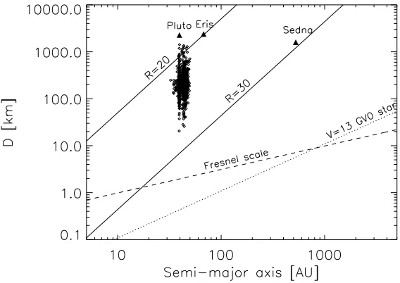
present occultation surveys). Figure 1.6 shows the region of diameter and

semi-major axis space where most TNOs reside. The current limit of direct observations

is shown at R = 30. The Fresnel scale is also shown: all objects that lay below

the dashed line would generate diffraction phenomena during an occultation. The

(27)

Figure 1.6: Diameter versus semi-major axis. The black diamonds show the known KBOs. The triangles indicate several of the larger, well-known outer Solar System objects at their semi-major axes. The solid lines indicate contours of constant brightness in reflected sunlight, assuming an albedo value of 0.04. The long dashed line shows the Fresnel scale

as a function of distance assuming λ= 650 nm. Occultations by objects below this line

are diffraction dominated. The dotted line is the angular size of a V=13 G0V star as a

function of distance. The limit of direct observations is shown atR = 30.

star becomes comparable to the Fresnel scale the diffraction features are smoothed

out (see Chapter 3 and Nihei et al. 2007).

1.4 The story told by the small KBOs

Probing the very small (D _≤ 10 km) region of the KBO size spectrum

and the regions of the solar system outside of the Kuiper belt could have profound

consequences on our understanding of the formation and on the evolution of the

solar system.

The Kuiper belt has been shaped by accretion and disruption processes

(28)

relative velocities of the objects in the early Kuiper belt were sufficiently low to

allow accretion processes to form kilometer and much larger objects. Later, when

the velocity dispersion increased as the KBO population was stirred up by the

grav-itational effects of the larger planets and planetoids, only large objects were able to

continue growing through impacts, whereas collisions among smaller bodies resulted

in disruption. The details of these processes depend on the internal strength of the

KBOs and on the orbital and dynamical evolution of the gas giant planets. The

size distribution of KBOs, therefore, contains information on the internal structure

and composition of the KBOs – and hence information on the location and epoch

in which they formed – and about planetary migration (Pan & Sari, 2005; Kenyon

& Bromley, 2004; Kenyon et al., 2008, and references therein).

Direct observations have detected KBOs as faint as magnitude R _∼ 28.2

(Bernstein et al., 2004), which corresponds to about 24 km in diameter assuming

a 4% albedo. The KBO size distribution can be characterized using its brightness

distribution. The latter is well described by a power law Σ(< R) = 10α(R−R0) _deg−2_,

with an index α = 0.6 and R0 = 23 (Fraser & Kavelaars 2008, Fuentes & Holman

2008) for objects brighter than about R = 25, or D _∼ 100 km. This is the

re-gion of the size spectrum which reflects the early history of agglomeration. Kenyon

& Windhorst (2001) pointed out that the intensity of the infrared Zodiacal

back-ground sets limits on the extrapolation of a straight power law to smaller sizes.

The relatively shallow size distribution of Jupiter Family Comets (JFCs, Tancredi

et al. 2006), which are believed to originate in the Kuiper belt, and the cratering

of Triton observed by Voyager 2 (Stern, 1996), all point to a flatter distribution

for small KBOs6_{. In 2004 evidence surfaced that a break in the power law occurs} 6

(29)

at a diameter larger than 10 km: Bernstein et al. (2004) conducted deep Hubble

Space Telescope observations with the Advanced Camera for Surveys which led to

the discovery of only 3 new objects fainter than R = 26, about 4% of the number

expected from a single power law distribution extrapolated to R = 29. While

this work remains the state of the art for deep direct surveys of the outer solar

sys-tem, recent campaigns have observed many more faint objects down to magnitude

R = 27, which with the assumption of a 4% albedo corresponds to about 40 km in

diameter7 _{(Fraser & Kavelaars 2008, Fuentes & Holman 2008, Fuentes et al. 2009b,}

and Fraser & Kavelaars 2009). These recent data allowed them to locate a break in

the power law size distribution in the diameter range D= 30₋120 km.

The range of the size spectrum of Kuiper belt objects (KBOs) between tens

of kilometers and meters in diameter is particularly interesting as models predict

here the occurrence of transitions between different strength and gravitation regimes

that would leave a signature in the size distribution (Pan & Sari 2005, Kenyon &

Bromley 2004, Benavidez & Campo Bagatin 2009, and references therein).

Occulta-tion surveys allow us to reach farther then the current limits of direct observaOcculta-tions,

and into this very region of interest, and they are the only observational method

presently expected to be able to detect such small objects in the outer solar system.

While occultation surveys were first proposed in 1976, only recently have

results been reported. This observational technique requires sub-second

photomet-ric measurements which have only recently become possible. Chang et al. (2006)

conducted a search for KBO occultations in the archival Rossi X-ray Timing

Ex-plorer (RXTE) observations of Scorpius-X1, the brightest X-ray source in the sky.

RXTE is a satellite dedicated to the observation of X-ray astronomical sources, able

7

(30)

to provides high cadence (_≥ µsec) time series of X-ray sources. Chang et al. (2006)

explored nearly 90 hours of Sco-X1 data collected between 1996 to 2002 by RXTE,

and reported a surprisingly high rate of occultation–like phenomena: dips in the

lightcurves compatible with occultations by objects between 10 and 200 m in

di-ameter. Jones et al. (2008) showed that most of the dips in the Sco-X1 lightcurves

may be attributed to artificial effects of the response of the RXTE photo-multiplier

after high energy events, such as strong cosmic ray showers. Only 12 of the original

58 candidates cannot be ruled out as artifacts, but are hard to confirm as events

(Jones et al., 2008; Chang et al., 2007; Liu et al., 2008). New RXTE/PCA data of

Sco X-1 provided a less constraining upper limit to the size distribution of KBOs

(Liu et al., 2008).

Several groups have conducted occultation surveys in the optical regime.

Roques et al. (2006) and Bickerton et al. (2008) independently observed narrow

fields at 45 Hz and 40 Hz, respectively, with frame transfer cameras. Such cameras

allowed them to obtain high signal-to-noise ratio (SNR) fast photometry on two stars

simultaneously. Both surveys expect a very low event rate due to the limited number

of stars and the limited exposure, and neither survey has claimed any detection of

objects in the Kuiper belt at this time8_{. An upper limit for KBOs with} _D_≥_{1 km}

was derived by Bickerton et al. (2008) by combining the non-detection result of the

surveys of Chang et al. (2007), Roques et al. (2006), and Bickerton et al. (2008).

In my graduate studies I participated in two campaigns to detect

occul-tation events in star time–series. This effort is described in the following chapters.

Chapters 2-4 describe the effort on the determination of the size distribution of

KBOs. The survey I conducted at the MMT with the Megacam imager is described

in Chapter 2. TAOS (Taiwanese American Occultation Survey) is a dedicated

auto-8

(31)

mated multi-telescope survey (Lehner et al., 2009b). TAOS reported no detections

but placed the strongest upper limit to date to the surface density of small KBOs,

which is reported in Zhang et al. (2008). My work on the first 3.75 years of TAOS

data, a substantially larger dataset than the one used in Zhang et al. (2008), is

de-scribed in Chapters 3 and 4. Chapter 5 describes a search in progress for Sedna-like

and scattered disk objects in the TAOS data. Finally I summarize the conclusions

(32)

Chapter 2 The sub-km end of the Kuiper

Belt size distribution

We conducted a search for occultations of bright stars by Kuiper belt

Ob-jects (KBOs) to estimate the density of sub-km KBOs in the sky. We report here the

first results of this occultation survey of the outer solar system conducted in June

2007 and June/July 2008 at the MMT Observatory using Megacam, the large MMT

optical imager. We used Megacam in a novel shutterless continuous–readout mode

to achieve high precision photometry at 200 Hz, which with point-spread function

convolution results in an effective sampling of_∼30 Hz. We present an analysis of 220

star hours at signal-to-noise ratio of 25 or greater. The survey efficiency is greater

than 10% for occultations by KBOs of diameter D_≥0.7 km, and we report no

de-tections in our dataset. We set a new 95% confidence level upper limit for the surface

density ΣN(D) of KBOs larger than 1 km: ΣN(D≥1 km) ≤ 2.0×108 deg−2, and

for KBOs larger than 0.7 km ΣN(D≥0.7 km) ≤ 4.8×108 deg−2.1

1

(33)

2.1 Introduction

The survey I report here was conducted using Megacam (McLeod et al.,

2006, Figure 2.2) at the 6.5 m MMT Observatory at Mount Hopkins, Arizona. The

use of Megacam in continuous–readout mode (see Section 2.2) on a field of view

of 24′ _×₂₄′ _{allowed us to monitor over} _∼ _{100 stars at 200 Hz over the course of}

two observational campaigns conducted in June 2007 and June-July 2008. This

peculiar use of a conventional CCD camera allowed us to reach the high speed

photometric sampling necessary to detect occultations by small outer solar system

objects without compromising the number of star targets monitored. Our survey is

0.4 km

5 km

Figure 2.1: A simulated diffraction pattern (left panel) generated by a sphericalD = 1 km

KBO occulting a magnitude 12 F0V star. The MMT/Megacam system bandpass (Sloan r’ filter and camera quantum efficiency) is assumed. The size of the KBO and the size of the Airy ring – a measure of the cross section of the event – are shown for comparison. The right panel shows the diffraction signature of the event (assuming central crossing: impact parameter b = 0) as a function of the distance to the point of closest approach (bottom scale). The top scale shows the time-line of the event assuming an observation

conducted at opposition (relative velocityv_rel = 25 km s−1_{). The occultation is sampled}

at 200 Hz (dashed line), and at 30 Hz, the effective sampling rate after taking PSF effects into account (solid line, see Section 2.3).

(34)

sensitive to occultations by outer solar system objects of diameter D _∼ 700 m or

larger.

In our survey, the bandpass of the observation is centered nearλ = 500 nm

and, at distance ∆ _∼ 40 AU, the Fresnel scale F isF _∼ 1.2 km. Any occultation

caused by objects in the Kuiper belt of a few kilometers in diameter or smaller

will exhibit prominent diffraction effects. Figure 2.1 shows a diffraction pattern

generated by a D = 1 km KBO (left) and the diffraction feature that would be

imprinted in a star lightcurve observed by our system (right).

We report no detections in 220 star hours. Our MMT survey is designed

2048 pixels

4608 pixels

x

y

Figure 2.2: Megacam focal plane (McLeod et al., 2006). A thick rectangle outlines a single CCD in the 9x4 CCDs mosaic. Two halves of each CCD (thin rectangles) are read into two separate amplifiers; each amplifier generates a separate output image in our observational

(35)

to be complementary to TAOS and to reach smaller size limits, and unlike TAOS

it would allow us to estimate the size of a detected occulting KBO. We expect

further work on adaptive photometry and de-trending to significantly improve our

sensitivity, perhaps allowing us to detect KBOs as small as D _≥ 300 m. I discuss

the improvements we are developing on this analysis in Section 6.1. The preliminary

analysis we present here allows us to derive upper limits for objects D_≥700 m.

In the next section I describe the novel observational mode adopted for

this survey. In Section 2.3 I describe the data acquired and analyzed for this paper.

Details of the data extraction and reduction, which required custom packages, are

addressed in the same section. Section 2.4 describes the characteristics of the noise

of our current datasets, and our noise mitigation approach. Section 2.5 describes

the detection algorithm. In Section 2.6 I derive our upper limit to the density of

KBOs. I also compare in detail the achievements of our survey to those of previous

surveys.

2.2 Fast Photometry with a Large telescope: The

Continuous – Readout Mode

Achieving sub-second photometric sampling is a challenge in optical

as-tronomy. CCD cameras can perform fast photometric observations by reading out

small sub-images, limiting the observations to very small portions of the sky (e.g.,

Marsh & Dhillon 2006, Bickerton et al. 2008). This is the approach adopted by

Roques et al. (2006), and Bickerton et al. (2008), who observed two stars at one

time. Due to the rarity of occultation events, however, one would want to maximize

the number of targets and the total exposure to increase the number of detections.

(36)

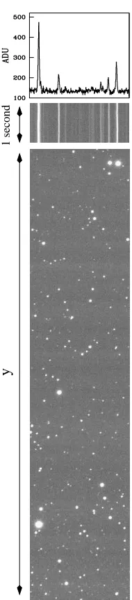
1 second

y

Figure 2.3: Conventional stare mode image (one half of a CCD) of one of our fields (bottom panel). A series of rows from continuous–readout mode (center panel) from the same CCD and field, where the rows are stacked together in a single image. The flux profile of the central row of this segment of continuous–readout data is plotted in the top panel.

zipper mode readout technique (Lehner et al., 2009b), but they sample at _≤ 5 Hz

rate. Our continuous–readout technique allows us to observe the entire field of view

of the camera at 200 Hz.

(37)

thirty-six CCDs – each with an array of 2048_×4608 pixels – with a 24′ _×₂₄′ _{field of}

view (Figure 2.2). The standard readout speed of each CCD is 0.005 sec/row with

2_×2 binning. For this survey, we operated the camera in shutterless continuous–

readout mode; that is, we kept the shutter open while scrolling and reading the

charges at the standard readout speed, tracking the sky at the sidereal rate. Each

star is represented in each row that is read out of the camera, and the flux from a

star in a row represents a photometric measurement of that star sampled at 200 Hz.

Stacking each read row into a single image each star time–series forms a streak along

the readout axis (y₋axis). A small portion of our data is shown in Figure 2.3.

In this observational mode the flux from the sky background is added

continuously as the charge is transferred from one end of the CCD to the other, so

the sky is exposed 2304_×0.005 = 11.52 sec for every 0.005 sec integration on each

star image (where 2304 is the effective number of rows in each 2_×2 binned CCD).

In this mode the photon limited SNR is typically _∼180 for anr′ _{magnitude 10 star.}

When observing multiple targets simultaneously one can notice that the

lightcurves are affected by common fluctuations, or trends, due for example to

weather patterns (Kim et al., 2008, and references therein). In our observational

mode, however, additional flux variations are caused by wind-induced resonant

oscil-lations of the telescope. While the image motion along thexaxis of the focal plane

(transverse to the readout direction) can be resolved (see Section 2.3.1), the image

motion parallel to the direction of the CCD readout induces an effective variation

in the exposure time of a star for a given row. These fluctuations are common to

all stars in the field (with possible position dependencies) and therefore, in

prin-ciple, they are completely removable. We discuss the de-trending of our data in

Section 2.3.1. Other sources of noise that affect continuous-readout mode data are

(38)

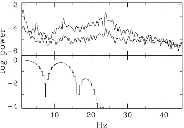
Figure 2.4: Top: power spectrum of one of our lightcurves before and after de-trending the lightcurve to remove noise (see Section 2.3.1). Bottom: power spectrum of the occultation

time–series for a 1 km KBO at 40 AU occulting a F0V V = 12 star.

minutes (after which the data load on the buffer would become prohibitive). For

each amplifier, a single FITS2 _{file is created wherein all of the rows read out during}

a data run are stored as a single image. For a typical run each FITS output image

contains 100K to 130K rows, corresponding to about 150–200 Mb of data.

2.3 Data

We selected observing fields within 2.8◦ _{of the ecliptic plane, where the}

concentration of KBOs is highest (Brown, 2001). In order to maximize the number

of targets we selected our fields at the intersection of the ecliptic and galactic planes

(RA _∼19h₀₀₀₀s_{, Dec} _{∼ −}₂₁o₀₀′₀₀′′_{). We conducted our observations in June-July,}

when our fields were near opposition (elongation angleε = 180◦_{) and the relative}

velocity of the KBOs is highest (Roques et al., 1987; Nihei et al., 2007; Bickerton

2

(39)

Table 2.1. MMT/Megacam survey observed fields

RA Dec λa _ε _rangeb

(deg) (deg)

17h₀₀₀₀s ₋₂₁◦₁₅′₀₀′′ _1.5 _174–160

17h₁₅₀₀s ₋₂₀◦₁₅′₀₀′′ _2.8 _176–163

18h₀₀₀₀s ₋₂₁◦₁₅′₀₀′′ _2.2 _171–173

18h₀₀₀₀s ₋₂₁◦₃₀′₀₀′′ _1.9 _171–173

18h₀₀₀₀s ₋₂₁◦₄₅′₀₀′′ _1.7 _172–173

19h₀₀₀₀s ₋₂₂◦₀₀′₀₀′′ _0.7 _158–172

a_{ecliptic longitude}

b_{range of elongation angles}

et al., 2009), thus maximizing the event rate per target star. Pointing information

for our fields is summarized in Table 2.1. The RA and Dec of each observed field

are listed together with the ecliptic latitude (λ) and a maximum range of elongation

angles at which the filed might have been observed.

We also observed control fields. These were chosen on the galactic plane

at a high ecliptic latitude; we expect a negligible rate of occultations by KBOs in

these fields. These data allow us to assess our false positive rate. Since we report no

detections the analysis of these fields is not discussed further in this paper. All of

our observations were conducted in Sloanr′_{filter (Smith et al., 2002). A set of about}

7 hours on target fields was collected in 5 half nights in June 2007 and a similar

number of hours was collected on control fields. A set of about 7 hours on target

fields and about 6 hours on control fields was collected in 7 half nights in June-July

2008. Out of the 2007 dataset 100.61 star hours at SNR _≥ 25 are considered in

this paper. From the 2008 dataset we use here 118.93 star hours. Information on

(40)

Table 2.2. MMT/Megacam survey data set parameters.

Start Date 2007 June 6

End Date 2007 June 10

Exposure at SN_≥25 100.61 star-hours

Number of lightcurves with SN_≥25 990 Number of Photometric Measurements 7.2_×107

Start Date 2008 June 27

End Date 2008 July 1

Exposure at SNR_≥25 118.93 star-hours

Number of lightcurves with SNR_≥25 527 Number of Photometric Measurements 8.5_×107

chosen arbitrarily: 25 is the minimum SNR of the surveys of Roques et al. (2006)

and Bickerton et al. (2008).3 _{A SNR 25 limits our sensitivity to fluctuations greater}

than 4%. An occultation of a magnitude 12 F0V star by a KBO of D = 400 m

diameter would produce a 4% effect. Our efficiency tests, however, revealed our

sensitivity rapidly drops below 10% for objects smaller than D = 700 m, due to

residual non-Gaussianity in our time–series photometric data. We discuss this in

Section 2.4.

2.3.1 Data extraction and reduction

Extraction

Custom algorithms have been developed for the data extraction and

re-duction. For each field a preliminary stare mode (conventional) image is collected

before each series of high-speed runs. At the beginning of our analysis the stare

3

(41)

mode image is analyzed using SExtractor (Bertin & Arnouts, 1996) to generate a

catalog of bright sources. This catalog is used to identify the initial position and

brightness of each star in the focal pane. In order to analyze the continuous readout

data, we first determine the sky background for each CCD and each row. To do

so we calculate the mean of the flux counts in each row after removing the

mea-surements that are three σ’s or more above the mean (3σ-clipping) iteratively until

the mean converges. This removes most of the pixels in the row containing flux

from resolved stars. Next, a subset of stars that are bright and isolated is selected

from the stare–mode catalog and used to determine the x-displacement of the focal

plane. The focal plane is split into two halves, 9_×2 chips each, that are analyzed

separately. We select eight stars, two near each of the four corners of each half-focal

plane. This allows us to characterize the global motion of the targets even in the

presence of small rotational modes or spatial dependency (see Section 2.4). For

each star (⋆), and at each time–stamp (t), we calculateµ⋆(t) and σ⋆(t), respectively

the centroid offset from the original position and the standard deviation of the star

image, assuming a Gaussian profile. Note that, for a given time-stamp, flux from

different stars will appear on different rows due to the y-positions of the stars on

the focal plane. A 1-D Gaussian

F⋆ = I⋆ exp

−(x−µ⋆(t))

2 2σ2

⋆(t)

+ Ibg (2.1)

(where F⋆ is the total star flux, I⋆ the flux at the peak and Ibg the sky) is fit for

each of the eight stars to each row of the star–streak. Thus thex-displacement ¯µ(t)

(42)

of the star displacements:

¯

µ(t) = 8

P

⋆=1

ω⋆(µ⋆(t)−µ⋆(t0))

8

P

⋆=1 ω⋆

, (2.2)

where µ⋆(t0) is the star initialx-position and ω⋆ is the weight used for that star.

In order to weight our average we use the correlation of the entire x–

displacement time–series µ⋆ with respect to the rest of the star set:

ω(i, j) = 1

T

X

t=0

(µi(t)− hµii)(µj(t)− hµji)

s2

i(t) s2j(t)

, (2.3)

ω⋆ =

1 7

X

j6=⋆

ω(⋆, j); (2.4)

wheres2 _{is the variance of the displacement throughout the duration}_T _{of the time–}

series. The weight ω⋆ is the square of the Pearson’s correlation coefficient (Rice,

2006, pag. 406), a measure of the correlation of the displacement time–series for

one star with the other seven. All star lightcurves in the field are then extracted

by aperture photometry adjusting time–stamp by time–stamp the center of the

aperture according to the x-motion derived in this stage, and with a fixed aperture

size which is proportional to the average FWHM in the run.4

De-trending

The lightcurves thus extracted show evident semi–periodic and quasi–

sinu-soidal flux variations that can be associated with oscillatory modes of the telescope

4

(43)

Figure 2.5: Image motion and PSF over time: mean of the x displacements for eight bright isolated stars, at the four corners of the half-focal plane for two data runs (top left and right panels). PSF width from the Gaussian fit averaged over the same set of stars (bottom left and right). On the left we used the same run used to generate Figure 2.8. The arrow points to the displacement feature marked in Figure 2.8. On the right the

x-displacement and the PSF width for another run, with the first 0.5 seconds shown on

the left at higher time resolution. Note how in the second run the x-displacements are

less prominent (note the differentyscale) but the amplitude of the variability of the PSF

is larger.

in the y direction. In particular, a Fourier analysis generally reveals two strong

modes, roughly consistent among runs, one with period near 0.04 seconds and the

other near 0.5 seconds. Fourier spectra for one of our lightcurves, before and after

processing it, are shown in Figure 2.4 (top). Because these fluctuations affect the

whole CCD plane, they are common to all stars and can be removed to achieve

greater photometric precision. We now want to identify and remove these trends

from our lightcurves, a process that we call de-trending.

The general algorithm we used for de-trending is described in Kim et al.

(2008). The method takes advantage of the correlation among lightcurves to extract

and remove common features. Since we can identify distinct semi–periodic modes

we de-trend high and low frequencies separately (typicallyν >10Hz andν < 10Hz).

We first smooth the lightcurves, to remove all but the frequencies that we

want to de-trend, by applying a low–pass or high–pass filter. We then select a subset

(44)

features. Nτ is typically about 15. A master trend lightcurve τ is generated as the

weighted average of the normalized template lightcurves:

τ(t) = 1

Nτ Nτ

P

j=1 σ2₍_f

τ,j) fτ,j(t)/hfτ,ji

Nτ

P

j=1 σ2₍_f

τ,j)

(2.5)

where the notation_hfτ,jidenotes the mean flux offτ,j(t) over the duration T of the

lightcurve, and the weightσ2₍_f

τ,j) is the variance of the lightcurve in time; τ(t) has

mean value of unity and it represents the correlated fluctuations in all lightcurves.

The main trend is physically associated with an over-under exposure

phe-nomenon due to global image motion along the y axis, which causes the effective

exposure time to vary (see Section 2.2), therefore scaling the flux. In order to remove

these common trends we divide point by point the flux of each original lightcurvef

by the trend master lightcurve. To improve the de-trending effectiveness we allow

a free multiplicative factor Af (a scaling factor) for each lightcurve as follows:

fd,Af(t) = f(t)

1

τ(t)−1

Af + 1

; (2.6)

fd,Af is the de-trended lightcurve.

We optimize our de-trending by selecting Af to minimize the variance of

the de-trended lightcurvefd with respect tofc = f−fs+hfsi, which is the original

lightcurve cleaned of the frequency to be de-trended. We apply a high–pass (low–

pass) filter to f to obtain fs if we want to de-trend the low (high) frequencies. Af

is then optimized by setting:

∂ ∂Af

T

X

t=1

fd,Af(t) − hfci

2

(45)

which minimizes the second moment of the de-trended lightcurve with respect tofc.

The optimal value of Af can be calculated analytically.

We set no constraints on Af, and for all of our runs the optimal values

of Af proved to be close to 1 (which is what we expect in the presence of global

trends) except for pathological cases where the flux of the star was buried in noise

and the raw and de-trended SNR were extremely low. These lightcurves would not

pass SNR cuts and were never considered in any of our analysis.

Examples of the results obtained by our de-trending algorithm are

dis-played in Figures 2.6 and 2.7. In Figure 2.6 the top two panels show lightcurves

for two independent sources in our field, and the bottom two panels show the same

lightcurves after de-trending. Note that the top star is _∼ 2.5 magnitudes brighter

than the other and this is reflected in the lower SNR of the fainter source (bottom

panel). Figure 2.7 shows one of our lightcurve before (top) and after de-trending

(bottom). The raw lightcurve is implanted with an occultation by a D = 1 km

KBO occulting a V = 9 F0V star. The diffraction feature is completely lost in the

trends and becomes evident only after de-trending. In the bottom panel we show

the lightcurve de-trended without allowing for the optimization factorAf at the top

(plotted at the top at an arbitrary offset) and with optimization factorAf = 1.15

for the low frequencies and Af = 1.05 for the high frequencies, shown at the

bottom. The introduction of an optimization factor improves the SNR of the

de-trended lightcurve from SNR = 30.0 to SNR = 30.7. For this particular run

improvements of up to 7% in SNR were achieved by optimizing the de-trending.

Note that, while we used smoothed versions of our lightcurves to identify

the trends and to optimize the de-trending, we do not smooth or filter our lightcurves

to improve the SNR, thus preserving all intrinsic features (including potential

(46)

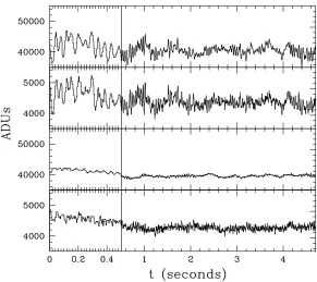
Figure 2.6: Lightcurves of two independent stars in one of our fields. The left-hand plots show a 0.5-second chunk of the time series; the following 4-seconds are shown on the right at a lower time resolution. The top two panels show the lightcurves before de-trending. Common modes are visible at multiple time scales. The bottom two panels show the lightcurves after de-trending. The top lightcurve is the same used in Figure 2.4

and after de-trending it (top). The power spectrum of an occultation time-series

generated by a 1 km KBO occulting a F0V star of magnitude V = 12 is shown

in the bottom panel. Our de-trending greatly reduced the power at all frequencies:

the cumulative power for this particular lightcurve at frequencies ν_≤40 Hz is

sup-pressed by a factor of 40. Because the oscillations are not perfectly correlated among

our stars (see Section 2.4) some residual power is visible. Smoothing however would

would significantly reduce the strength of the occultation features, that show power

(47)

Figure 2.7: Raw lightcurve on which the occultation signature of a 1 km KBO

occult-ing a magnitude V = 9 F0V star has been implanted (top) and the same lightcurve

after de-trending (bottom). In the bottom panel the top lightcurve is de-trended without optimization (plotted at the top at an arbitrary offset) and the bottom lightcurve is

de-trended with optimization factorA_f = 1.15 for the low frequencies and 1.05 for the high

frequencies.

2.4 Residual noise in the time-series

With a SNR & 25 we can detect fluctuations of a few–percent. In an

0.005 sec exposure the flux for a magnitude r′ _{= 14 star observed by Megacam is}

about 103 _e−_{, which after taking into account the contribution to the noise of the}

background should lead to a Poisson limited SNR of about 25. While we were able

to remove a large portion of the noise that originally affected our data, we typically

cannot reach the Poisson-limit. We have identified five possible sources of noise in

our data:

• Contamination by nearby sources. Overlap of stars along the xaxis

(per-pendicular to the read-out direction) within a chip, causes reciprocal

(48)

compromised and excluded from our analysis. Furthermore, oscillations of the

images along the x axis causes the relative distance between the star–streaks

to change, which causes occasional merging. Note that while these oscillations

are simultaneous in time domain, they do not occur in the same row in the

recorded image. In each row the star images of two objects that are at a

dif-ferent y position on the CCD plane will not belong to the same time-stamp,

therefore the oscillations – while simultaneous – will show a y offset. This is

shown in Figure 2.8. The merging of streaks causes artificially high counts.

Aperture photometry with a fixed aperture does not address this issue properly

and fitting photometry on individual streaks is a computationally expensive,

inefficient method which is also unstable in the presence of multiple sources

close to each other.

• Unresolved sources. Sources that are too faint to be visible in our 0.005

sec exposures generate a diffuse background. For the data in Figure 2.3 the

sky level calculated as the 3σ₋clipped mean of the row counts is 140.5 ADUs.

The stare mode image sky level was 48 ADUs for a 5 sec exposure, which

would lead to a prediction of 110 ADUs for our 0.005 _×2304 sec effective

continuous–readout exposure. The discrepancy is due to the presence of

un-resolved streaks associated with faint stars across the field. Summing all the

counts in the stare mode image and rescaling by the exposure time of each row

we get a number very close to the sum of all counts in a row of

continuous-readout data. This contamination introduces extra Poisson noise, but more

importantly it introduces non-Poissonian noise as well, since the unresolved

sources are affected by the same trends the bright stars display. Our data

shows evidence of off–phase correlation that might be induced by unresolved

Chasing Shadows in the Outer Solar System

University of Pennsylvania

ScholarlyCommons

Chasing Shadows in the Outer Solar System

Federica Bianco

Chasing Shadows in the Outer Solar System

CHASING SHADOWS IN THE OUTER SOLAR SYSTEM

Federica Bianco

Acknowledgments

ABSTRACT

Contents

List of Tables

List of Figures

Chapter 1

Introduction

1.1

Historical note

1.2

Formation

1.3

Observational techniques to explore the outer

solar system

1.3.1

Diffraction dominated occultations of bright stars

1.4

The story told by the small KBOs

Chapter 2

The sub-km end of the Kuiper

Belt size distribution

2.1

Introduction

0.4 km

5 km

2048 pixels

4608 pixels

x

y

2.2

Fast Photometry with a Large telescope: The

Continuous – Readout Mode

2.3

Data

2.3.1

Data extraction and reduction

2.4

Residual noise in the time-series