www.nat-hazards-earth-syst-sci.net/14/525/2014/ doi:10.5194/nhess-14-525-2014
© Author(s) 2014. CC Attribution 3.0 License.
Natural Hazards
and Earth System
Sciences
Application of GA–SVM method with parameter optimization for
landslide development prediction
X. Z. Li1,2and J. M. Kong1,2
1Key Laboratory of Mountain Hazards and Surface Process, Chinese Academy of Sciences, 610041, Chengdu, China 2Institute of Mountain Hazards and Environment, Chinese Academy of Sciences, 610041, Chengdu, China
Correspondence to: J. M. Kong ([email protected]) and X. Z. Li ([email protected])
Received: 21 August 2013 – Published in Nat. Hazards Earth Syst. Sci. Discuss.: 8 October 2013 Revised: 28 December 2013 – Accepted: 22 January 2014 – Published: 4 March 2014
Abstract. Prediction of the landslide development process is always a hot issue in landslide research. So far, many methods for landslide displacement series prediction have been proposed. The support vector machine (SVM) has been proved to be a novel algorithm with good performance. How-ever, the performance strongly depends on the right selec-tion of the parameters (C andγ) of the SVM model. In this study, we present an application of genetic algorithm and support vector machine (GA–SVM) method with parameter optimization in landslide displacement rate prediction. We selected a typical large-scale landslide in a hydro-electrical engineering area of southwest China as a case. On the basis of analyzing the basic characteristics and monitoring data of the landslide, a single-factor GA–SVM model and a multi-factor GA–SVM model of the landslide were built. More-over, the models were compared with single-factor and multi-factor SVM models of the landslide. The results show that the four models have high prediction accuracies, but the ac-curacies of GA–SVM models are slightly higher than those of SVM models, and the accuracies of multi-factor models are slightly higher than those of single-factor models for the landslide prediction. The accuracy of the multi-factor GA– SVM models is the highest, with the smallest root mean square error (RMSE) of 0.0009 and the highest relation in-dex (RI) of 0.9992.
1 Introduction
Prediction of the landslide development process is a critical task in landslide research (Sornette et al., 2004; Helmstetter et al., 2004; Corominas et al., 2005; Gao, 2007). Accurate
prediction can provide a scientific guide to landslide pre-warning and forecast and engineering control as quickly as possible. However, it is not easy to accurately predict the evolution behavior of landslides. This is mainly because of geometrical complexity, nonlinearity of the displacement– time relationships and a large number of interplaying factors, hardly taken into account by prediction models (Crosta and Agliardi, 2002).
The most common method of predicting the development process is to build suitable models according to the de-velopment mechanism and monitoring data of landslides. So far, many models have been put forward (Saito, 1965; Voight, 1989; Crosta and Agliardi, 2002; Lu and Rosenbaum, 2003; Feng et al., 2004; Helmstetter et al., 2004; Neau-pane and Achet, 2004; Sornette et al., 2004; Randall, 2007; Mufundirwa et al., 2010). They can be roughly classified into four categories: deterministic physical models, statistics models, nonlinear models and numerical simulation models (Li et al., 2012). Among them, the nonlinear models are con-sidered to have the greatest potential for coping with difficult and complicated problems. Especially, artificial intelligence methods represented with neural networks (NNs) have been widely used in landslide prediction recently (Lu and Rosen-baum, 2003; Neaupane and Achet, 2004). However, some problems have appeared in the practical applications of NN methods because of imperfect theory, such as being suitable only for large data sets and having both easily occurring lo-cal minimum and weak generalization ability. Therefore, we need to find a better method for landslide development pre-diction.
co-workers. The method works on Vapnik–Chervonenkis (VC) dimension theory of statistic learning theory (SLT) and structural risk minimization principle (Cortes and Vapnik, 1995). It seeks an optimal compromise between the com-plexity (the learning accuracy for certain training samples) and learning capacity (the predicting ability for any other samples) of models according to limited samples, in order to obtain the best generalization ability (Cortes and Vapnik, 1995; Cristianini and Shawe-Taylor, 2000). It can preferably resolve problems with small samples, and nonlinear and high dimensions. Hence, the method has been widely used in the fields of classification and regression (Oliveira et al., 2004; Khan et al., 2006). Recently, a few researchers have begun to try to apply the method in landslide and slope research. For example, Yao et al. (2008), and Ballabio and Sterlacchini et al. (2012) applied it to landslide susceptibility mapping and assessment and obtained good results. Samui (2008) used it to predict safety status and factors of slopes, and indicated that the SVM model gives a better result than the result of artificial neural networks (ANNs) for safety factor prediction of slopes.
Although SVM theory has been widely used in some fields, its application results do not reach the expected re-sults of the theory. According to the related references (Cherkassky and Ma, 2004; Lessmann et al., 2005; Min and lee, 2005), the selection of kernel functions and parameters is one of main factors affecting the application results. At present, parameters of the SVM model are manually selected by experience, there being lack of a guide of mature theory. Genetic algorithm (GA) is a global optimization algorithm with good robustness, which was first suggested by John Holland in 1975 (Goldberg and Holland, 1988). GA can be used to automatically recognize some parameters of SVMs (Lessmann et al., 2005; Pourbasheer et al., 2009). Hence, we present an application of GA–SVM in landslide development prediction.
The paper is organized as follows: Sect. 1 starts with liter-ature associated with landslide development prediction and features and applications of related prediction methods. tion 2 introduces the SVM, GA and GA–SVM methods. Sec-tion 3 presents a typical large-scale landslide case. Applica-tion results are described in Sect. 4. Discussion and conclu-sions are presented in Sect. 5.
2 Methodology
2.1 SVM for regression
As the detailed description of SVM theory can be found in various references (e.g., Cortes and Vapnik, 1995; Cristianini and Shawe-Taylor, 2000), here we only introduce some key points of SVM for regression (SVMR).
SVMR has two types: linear regression and nonlinear re-gression. For linear regression, first consider the problem
us-ing a linear regression function
f (x)=ω·x+b (1) to fit the data{xi, yi},i=1,2, . . . , n,xi∈Rn,yi∈R, where ωis an adjustable weight vector,bis scalar threshold,xis the input andy is the output,Rnisn-dimensional vector space andR is one-dimensional vector space. In order to find a function as flat as possiblef (x)that gives a deviationεfrom the actual output (y), a smallestωwould need to be found. It can be obtained by minimizing the Euclidean normkωk2 (Smola and Scholkopf, 2004; Samui, 2008). This can be writ-ten into a convex optimization problem as follows:
Minimize: 1 2kωk,
Subject to:
yi− hω·xii −b≤ε hω·xii +b−yi≤ε
(i=1,2, . . . , n). (2) Considering the existence of some permissible error, slack variablesξiandξi∗are introduced into the above optimization problem. Equation (2) becomes
Minimize: 1
2kωk +C n X
i=1
(ξi+ξi∗),
Subject to:
yi−hω·xii −b≤ε+ξi hω·xii+b−yi≤ε+ξi∗
ξi, ξi∗≥0
(i=1,2, . . . , n), (3)
where the constantC >0 shows the penalty degree of the sample with error exceedingεand is called a penalty factor.
A dual problem of Eq. (3) can be obtained by using the optimization method.
Maximize:W a,a∗ = −1
2 n X i,j=1
ai−ai∗
aj−a∗j
xi·xj
+ n X i=1
yi ai−ai∗
−ε
n X i=1
ai+ai∗
,
Subject to: n P i=1
ai−a∗i
=0
ai ≥0
ai∗≤C
i=1,2,· · ·, n, (4)
whereaiandai∗are Lagrange multipliers.
Solving the above optimization problem, the fitness func-tion of SVM can be given by
f (x)=ω·x+b= k X
i=1
ai−a∗i
wherek is the number of support vectors, and the samples (xi, yi)corresponding toai−ai∗6=0 are support vectors.
For the nonlinear problem, the origin problem can be mapped into a high-dimensional feature space by some nonlinear transformation (Cristianini and Shawe-Taylor, 2000). In the feature space, the inner product operation of linear problem can be substituted by kernel functions, i.e.,K xi,xj
= ∅(xi)· ∅(xj). Therefore, Eqs. (4) and (5) can be written as
Maximize:W a,a∗ = −1
2
n
X
i,j=1
ai−ai∗
aj−aj∗
K xi,xj
+
n
X
i=1
yi ai−ai∗
−ε
n
X
i=1
ai+ai∗
,
Subject to: n P i=1
ai−a∗i
=0
ai≥0
ai∗≤C
i=1,2, . . . , n , (6)
f (x)=ω·x+b= k X i=1
ai−a∗i
K xi,xj+b, (7)
whereK xi,xjis a kernel function that measures the sim-ilarity of distance between the input vectorxi and the stored training vectorx(Feng et al., 2004). The meanings of other parameters are same as for the parameters mentioned above. At present, four basic kernel functions have been widely used. They are (Cristianini and Shawe-Taylor, 2000)
– linear:K(xi,xj)=(xi,xj).
– polynomial:K(xi,xj)= [γ·(xi,xj)+1]d,γ >0. – radial basis function (RBF):
K(xi,xj)=exp
−γ·xi−xj
2 .
– sigmoid kernel:K(xi,xj)=tanh[γ (xi,xj)+r]. Here,γ,r, andd are kernel parameters. In this study, we mainly used RBF as kernel function of the SVM model for landslide prediction, because the function has strong nonlin-ear mapping ability.
2.2 Genetic algorithm (GA)
GA, an adaptive optimizing method with overall searching function, was devised by simulating the genetic evolution mechanism of biology in the natural environment (Whit-ley, 1994). The method simulates the copying, crossing and variation phenomena in the process of natural selection and heredity. Starting from any initial population, a group of new better-adapted individuals can be generated by randomly selecting, crossing and variation operations. Therefore, by
unceasing evolution from generation to generation, a best-adapted individual (the optimal solution of the optimal prob-lem) can be acquired at last. It has the advantages of global optimality, implicit parallelism, high stability and wide us-ability. The method has been widely used in computer sci-ence, engineering management and social science (Lessmann et al., 2005; Pourbasheer et al., 2009; Choudhry and Garg, 2009). In this study, we mainly use GA to search for the pa-rameters (Candγ) of the SVM model for landslide develop-ment prediction.
2.3 GA–SVM model
In order to build an effective SVM model, the parameters (C
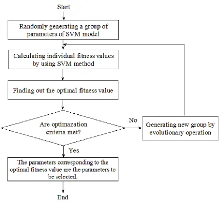
andγ) of the model need to be chosen properly in advance (Lin, 2001). The parameterC determines the tradeoff cost between minimizing the training error and complexity of the SVM model. With a biggerCvalue, the predictive accuracy of the training sample is higher. However, this may cause an over-training problem. The parameterγ of the RBF ker-nel function defines a nonlinear mapping from input space to high-dimensional feature space. The value ofγ affects the shape of RBF function. Hence, the parameters (C andγ) have a powerful influence on the efficiency and generaliza-tion performance of the SVM model. At present, the choice of the parameters lacks the guide of mature theory, mainly depending on experiences. A grid-search technique was pre-sented by Lin (2001). However, the grid algorithm is time consuming and does not perform very well (Gu et al., 2011). According to some related research in different fields, GA is proved to be a better choice to determine the parameters (Lessmann, 2005; Pourbasheer et al., 2009). It can reduce the blindness of human-made choice and improve the predicative performance of the SVM model. Therefore, we choose GA to search for the optimal parameters of the SVM model for landslide prediction in this study. The basic flowchart of the GA–SVM method can be seen in Fig. 1.
The algorithm can be realized by a parameter optimization procedure designed by Y. Li of Beijing Normal University based on the libsvm-mat toolbox, which was developed by Lin of National Taiwan University (Chang and Lin, 2001).
3 Landslide case study
Here, we selected a typical large-scale landslide in southwest China as a case.
3.1 Basic characteristics of the landslide
Fig. 1. Basic flowchart of GA–SVM method.
The slope direction is 210–215◦. The landslide body borders 1400 m elevation, the terrain below the elevation of 1400 m is gentle, with an average gradient of 22–25◦; while the terrain above the elevation of 1400 m is steeper, with a gradient of 35–45◦. The landslide has three free faces, and there are sev-eral gullies and multi-level gentle slopes on the uneven slope face (Fig. 2).
The upper part of the landslide body is composed of basalt with blocky structure; its lower part is composed of lay-ered sedimentary rock. The landslide body can be divided into three zones from upstream to downstream, according to lithology and material composition characteristics and the continuity of the slip surface. Zone I, an ancient landslide area, is located in the upstream side of the landslide, with a trench and valley landform. Zone II, a creep area of rock that is the main deformation area of the landslide, is located in the middle of the landslide, with a ridge landform. Zone III, a shallow-surface landslide area, is located in the downstream
side of the landslide, with a ridge landform (Fig. 2). Our re-search focus is on Zone II.
3.2 Monitoring data of the landslide
Fig. 2. The whole view of the landslide.
the landslide body of Zone II, 110 monitoring points were set up, including 11 monitoring points of surface displace-ment, 4 drilling monitoring points for observing deep dis-placement of the landslide and groundwater temperature and level, 49 monitoring points for vertical and horizontal dis-placements of two footrill soleplates, 7 monitoring points for groundwater flow and temperature in the footrills, and 39 crack monitoring points for surface and buildings. The system with large scale, high accuracy and many items was at the industry leading standard at that time. In order to en-sure sufficient accuracy, monitoring instruments are always regularly serviced and renewed, and intensive observations were made after the reservoir impounding. So far, we have accumulated a large amount of detailed monitoring data for the landslide. The long-term and continuous monitoring data provide a good basis for studying in detail the deformation law and mechanism of the landslide.
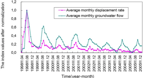
In this study, we choose the footrill monitoring data of the creep body in Zone II from April 1998 to December 2005 to deeply analyze the relationships between the landslide dis-placement rate and rain, reservoir water and groundwater. The displacement rate is calculated on the basis of the mon-itoring displacement values. For contrast, the index values are normalized by the min–max normalization method. The method performs a linear transformation on the original data. Suppose that minaand maxaare the minimum and maximum values for attributeA. The method maps a valuevof A tov0
in the range [0, 1] by computing
v0=(v−mina)/(maxa−mina). (8) The analysis results of the landslide are shown in Figs. 3–5 after using the above transformation.
Figure 3 shows that there is a good relationship between landslide displacement rate and rainfall, and the peaks of the displacement rate generally lag behind the rainfall peaks. As can be seen from Fig. 4, the impact of reservoir water level
Fig. 3. The relationship between the displacement rate and rainfall for the landslide.
Fig. 4. The relationship between the displacement rate and reservoir water level for the landslide.
Fig. 5. The relationship between the displacement rate and ground-water flow for the landslide.
displacement rate. They were consistent and reached peak levels at almost the same time.
Based on the above analysis results and the engineering geological survey results, the development process of the landslide is affected by rain and reservoir water as well as by other factors. However, the deformation is mainly affected by rainfall conditions, except that the changes of reservoir water level also had a powerful effect on the landslide in the early stages of storing water.
4 Application results
In this section, we analyze the development of the land-slide, based on the above-mentioned GA–SVM method and the monitoring data analysis results. We respectively built a single-factor GA–SVM model and a multi-factor GA–SVM model for the landslide.
4.1 Single-factor GA–SVM prediction result
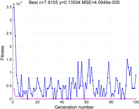
Firstly, we take the average monthly displacement rate of the landslide from April 1998 to December 2005 (93 data points) as a factor for building model. The earliest 62 data points were chosen as training samples, and the other 31 were considered as test samples. We built a single-factor SVM model for the landslide development prediction, and deter-mined the parameters (C andγ) of the model by GA. The GA had a generation number of 100, population size of 20. The search range of C andγ parameters is [0, 100]. The process-searched optimal parameters by GA can be seen in Fig. 6. We obtained a bestCparameter of 7.9155, and a best
γparameter of 0.13504. The model with the best parameters has the smallest mean square error (MSE). The prediction result of the GA–SVM model with the optimal parameters is shown in Fig. 7.
Figure 7 shows that the monitoring data are in good agree-ment with the prediction result of the single-factor GA–SVM model.
4.2 Multi-factor GA–SVM prediction result
Secondly, we take the average monthly displacement rate, erage monthly reservoir water level, monthly rainfall and av-erage monthly groundwater flow of the landslide from April 1998 to December 2005 as main factors for building a model. Similarly, the earliest 62 data points of the four factors were chosen as training samples, and the other 31 data points of the four factors were considered as test samples. We also built a multi-factor SVM model for the landslide develop-ment prediction, and determined the parameters (C andγ) of the model by GA. The parameters of GA and the search range of C andγ parameters are identical to those of the single-factor GA–SVM. The process of obtaining the param-eters and the prediction results of this model can be seen in Figs. 8 and 9.
Fig. 6. The fitness curve of searching for the optimal parameters of the single-factor SVM by GA.
Fig. 7. The curves of the monitoring and predicting values of the displacement rate of the landslide with time.
Figure 9 also shows that the monitoring data have good agreement with the prediction result of the multi-factor GA– SVM model.
4.3 Comparison of GA–SVM and SVM prediction results
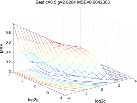
In order to evaluate the prediction performance of the above GA–SVM models, we also built single-factor and multi-factor SVM models of the landslide by using the same training samples as the GA–SVM models, and obtained the model parameters (Candγ) by using the grid-search method (Figs. 10 and 11).
Fig. 8. The fitness curve of searching for the optimal parameters of the multi-factor SVM by GA.
Fig. 9. The curves of the monitoring and predicting values of the displacement rate of the landslide with time.
Generally, the smaller the RMSE and the higher the RI, the higher the accuracy of the model is. They can be calculated by using the following formulas (Li et al., 2012):
RMSE= v u u u t
n P k=1
(X(0)(k)− ˆX(0)(k))
n , (9)
RI= v u u u u u u t
1− n P k=1
(X(0)(k)− ˆX(0)(k))2 n
P k=1
(X(0)(k)− ¯X(0))2
, (10)
whereX(0)(k)is the observed value andXˆ(0)(k)is the pre-dicted value of the models, andnandX¯(0) are the size and average value of the data sequenceX(0)(k).
Fig. 10. The 3-D contour map of the parameter selection of the single-factor SVM model by using grid-search method.
Fig. 11. The 3-D contour map of the parameter selection of the multi-factor SVM model by using grid-search method.
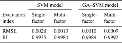
The prediction accuracy indexes of the models are shown in Table 1. As can be seen from Table 1, the prediction mod-els have very high accuracies, with the RI values relating the predicting and monitoring values reaching 0.99. The accu-racies of GA–SVM models are slightly higher than those of SVM models, and the accuracies of multi-factor models are slightly higher than those of single-factor models. Among the models, the accuracy of the multi-factor GA–SVM mod-els is the highest, with the smallest RMSE of 0.0009 and the highest RI of 0.9992.
5 Discussion and conclusions
Table 1. The accuracy comparison of the SVM and GA–SVM mod-els for the landslide.
SVM model GA–SVM model
Evaluation Single- Multi- Single- Multi-index factor factor factor factor
RMSE 0.0026 0.0013 0.0010 0.0009 RI 0.9935 0.9984 0.9989 0.9992
high-dimensional problems. It works on the VC dimen-sion theory of statistic learning theory and structural risk minimization principle (Cortes and Vapnik, 1995). It can obtain a very complex nonlinear mapping relationship of independent and dependent variables through the learning of training samples. Moreover, it is a learning method based on small samples. Building a model to using it does not need too many training samples. It is different from traditional statistics theory and artificial neural network methods, which are suitable for big samples (the sample size approaches infinity). Comparing the methods, the SVM method has a solid theory foundation, easily deals with high-dimensional and nonlinear problems, and can avoid local minimum and dimension disaster problems in ANN methods. The disadvantage of the method mainly lies in its complicated theory. For the purpose of a wide application, some researchers have developed some toolboxes for the SVM method, such as the libsvm toolbox (Chang and Lin, 2001).
Despite the above advantages, the generalization perfor-mance of the SVM models strongly depends on the right choice of its kernel functions and the parameters (C andγ) (Cherkassky and Ma, 2004; Lessmann et al., 2005). Hence, it is vitally important to reasonably determine them. GA is an adaptive optimizing method with overall searching function. In order to avoid the blindness of the parameter selection of the SVM model, we select GA to automatically search for the parameters of the model for landslide prediction.
In this study, we took a complicated large-scale landslide in a hydro-electrical engineering area of southwest China as a case. The landslide is located in the upstream reach of a hydropower station. Its development process is affected by many factors, such as rain, reservoir water, groundwater and human activity as well as the natural features of the landslide body. Moreover, the factors interrelate and interact with each other. We present an application of the GA–SVM method with parameter optimization in landslide displacement rate prediction. GA and SVM are organically combined by using GA to automatically search for the parameters of the single-factor and multi-single-factor SVM models of the landslide.
In addition, we also built the single-factor and multi-factor traditional SVM models of landslide prediction. By compar-ing, we find that the accuracies of the GA–SVM models are slightly higher than those of the SVM models, and the
accu-racies of multi-factor models are slightly higher than those of single-factor models for landslide prediction. Among the models, the accuracy of the multi-factor GA–SVM models is the highest, with the smallest RMSE of 0.0009 and the biggest RI of 0.9992.
The application results indicate that SVM and GA–SVM models have good prediction performance for landslide de-velopment tendency, and GA is an effective way for the se-lection of parameters of the SVM models. Because of the complexity of landslides and diversity and randomness of factors that influence them, the application of SVM and GA– SVM methods in the landslide development prediction has significant potential.
Acknowledgements. This research is supported by National Key Basic Research Program of China (no. 2013CB733205), Key Deployment Research Program of CAS (no. KZZD-EW-05-01-02), the National Natural Science Foundation of China (no. 40802072) and Key Research Program of Key Laboratory of Mountain Haz-ards and Surface Process, CAS (no. Y3K2040040). The authors wish to thank H. B. Havenith and one anonymous referee for their constructive comments. Special thanks are given to David Keefer for his helpful advice and great help in the linguistic improvement of English.
Edited by: D. Keefer
Reviewed by: H.-B. Havenith and one anonymous referee
References
Ballabio, C. and Sterlacchini, S.: Support Vector Machines for Landslide Susceptibility Mapping: The Staffora River Basin Case Study, Italy, Math. Geosci., 44, 47–70, 2012.
Chang, C. C. and Lin, C. J.: LIBSVM: a library for support vector machines, ACM Trans. Int. Syst. Technol., 2, 1–39, 2001. Cherkassky, V. and Ma, Y.: Practical selection of SVM parameters
and noise estimation for SVM regression, Neural Networks, 17, 113–126, 2004.
Choudhry, R. and Garg, K.: A hybrid machine learning system for stock market forecasting, World Academy of Science, Eng. Tech-nol., 39, 315–318, 2009.
Corominas, J., Moya, J., Ledesma, A., Lloret, A., and Gili, J. A.: Prediction of ground displacements and velocities from ground-water level changes at the Vallcebre landslide (Eastern Pyrenees, Spain), Landslides, 2, 83–96, 2005.
Cortes, C. and Vapnik, V.: Support-vector networks, Machine Learning, 20, 273–297, 1995.
Cristianini, N. and Shawe-Taylor, J.: An introduction to support vector machines and other kernel-based learning methods, Cam-bridge university press, 2000.
Crosta, G. B. and Agliardi, F.: How to obtain alert velocity thresh-olds for large rockslides, Phys. Chem. Earth, 27, 1557–1565, 2002.
Gao, W.: Study on displacement prediction of landslide based on grey system and evolutionary neural network, Comput. Methods Eng. Sci., 275–275, doi:10.1007/978-3-540-48260-4_121, 2007. Goldberg, D. E. and Holland, J. H.: Genetic algorithms and machine
learning, Machine Learning, 3, 95–99, 1988.
Gu, J., Zhu, M., and Jiang, L.: Housing price forecasting based on genetic algorithm and support vector machine, Expert Syst. Appl., 38, 3383–3386, 2011.
Helmstetter, A., Sornette, D., Grasso, J. R., Andersen, J. V., Gluz-man, S., and Pisarenko, V.: Slider-Block Friction Model for Landslides: Application to Vaiont and La Clapiere Landslides, J. Geophys. Res., 109, 1–15, 2004.
Khan, M. S. and Coulibaly, P.: Application of Support Vector Ma-chine in Lake Water Level Prediction, J. Hydrol. Eng., 11, 199– 205, 2006.
Lessmann, S., Stahlbock, R., and Crone, S. F.: Optimizing hyper-parameters of support vector machines by genetic algorithms, In IC-AI, 74–82, 2005.
Li, X. Z., Kong, J. M., and Wang, Z. Y.: Landslide displacement prediction based on combining method with optimal weight, Nat. Hazards, 61, 635–646, 2012.
Lin, P. T.: Support vector regression: Systematic design and perfor-mance analysis, Unpublished Doctoral Dissertation, Department of Electronic Engineering, National Taiwan University, 2001. Lu, P. and Rosenbaum, M. S.: Artificial neural networks and grey
systems for the prediction of slope stability, Nat. Hazards, 30, 383–398, 2003.
Marjanovic, M., Kovacevic, M., Bajat, B., and Vozenilek, V.: Land-slide susceptibility assessment using SVM machine learning al-gorithm, Eng. Geol., 123, 225–234, 2011.
Min, J. H. and Lee, Y. C.: Bankruptcy prediction using support vec-tor machine with optimal choice of kernel function parameters, Expert Syst. Appl., 28, 603–614, 2005.
Mufundirwa, A., Fujii, Y., and Kodama, J.: A new practical method for prediction of geomechanical failure-time, Int. J. Rock Mech. Mining Sci., 47, 1079–1090, 2010.
Neaupane, K. M. and Achet, S. H.: Use of backpropagation neu-ral network for landslide monitoring: a case study in the higher Himalaya, Eng. Geol., 74, 213–226, 2004.
Oliveira, L. S. and Sabourin, R.: Support Vector Machines for Handwritten Numerical String Recognition, Ninth International Workshop on Frontiers in Handwriting Recognition, 39–44, 2004.
Pourbasheer, E., Riahi, S., Ganjali, M. R., and Norouzi, P.: Applica-tion of genetic algorithm support vector machine (GA-SVM) for prediction of BK-channels activity, Euro. J. Medicinal Chem., 44, 5023–5028, 2009.
Randall, W. J.: Regression models for estimating coseismic land-slide displacement, Eng. Geol., 91, 209–218, 2007.
Saito, M.: Forecasting the time of occurrence of a slope failure, Pro-ceedings of the 6th International Conference on Soil Mechanics and Foundation Engineering, Montréal., Que, Pergamon Press, Oxford, 537–541, 1965.
Samui, P.: Slope stability analysis: a support vector machine ap-proach, Environ. Geol., 56, 255–267, 2008.
Smola, A. J. and Scholkopf, B.: A tutorial on support vector regres-sion, Stat. Comput., 14, 199–222, 2004.
Sornette, D., Helmstetter, A., Andersen, J. V., Gluzman, S., Grasso, J. R., and Pisarenko, V.: Towards landslide predictions: two case studies, Phys. A, 338, 605–632, 2004.
Voight, B.: A relation to describe rate-dependent material failure, Science (Washington, DC), 243, 200–203, 1989.
Whitley, D.: A genetic algorithm tutorial, Stat. Comput., 4, 65–85, 1994.