L
p
Loss Functions in Invariance Alignment and
Haberman Linking
Alexander Robitzsch1,2*
1 IPN – Leibniz Institute for Science and Mathematics Education, Kiel, Germany
2 Centre for International Student Assessment (ZIB), Kiel, Germany
* Correspondence: [email protected]
Abstract:The comparison of group means in latent variable models plays a vital role in empirical research in the social sciences. The present article discusses extensions of invariance alignment and Haberman linking concerning the choice of linking functions for comparisons of many groups. Robust linking functions are proposed for invariance alignment and robust Haberman linking that are particularly suited to item response data under partial invariance. In a simulation study, it is shown that both linking approaches have comparable performance, and in some conditions, the newly proposed robust Haberman linking outperforms invariance alignment.
Keywords: factor model, 2PL model, linking, invariance alignment, Haberman linking, partial invariance, item response model, structural equation model, differential item functioning
1. Introduction
In the comparison of multiple groups in latent variable models like factor analysis or item response models, some identifying assumptions have to be posed. In practice, it is often assumed that item parameters are equal across groups, which is denoted as invariance. The invariance concept has been very prominent in psychology and the social sciences in general [1,2]. For example, in international large-scale assessment studies in education like the programme for international student assessment (PISA), the necessity of invariance is strongly emphasized [3].
In the violation of invariance, linking approaches have been proposed to allow group comparisons. In this article, two important linking approaches are compared: invariance alignment [4] and Haberman linking [5]. These two approaches are contrasted by introducing a unifying notation. Moreover, these approaches are extended by considering a broad family of linking functions, theLploss function. By means of this extension, invariance alignment and Haberman linking appear to be very similar on a formal level, and through a simulation study it is shown that they provide comparable results.
2. Unidimensional Factor Model with Partial Invariance
In this section, the unidimensional factor model for continuous and dichotomous items for multiple groups (i.e., multiple populations) is introduced. Afterward, different assumptions about levels of invariance of item parameters are discussed.
2.1. Unidimensional Factor Model
LetXigdenote the item response variable of itemi
(
i=
1, . . . ,I)
in groupg(
g=
1, . . . ,G)
. For continuous itemsXig, a unidimensional factor model is assumed [6]Xig
=
νig+
λigθg+
εig , θg∼
N(
µg,σg2)
, εig∼
N(
0,ψig)
, (1)whereλigare item loadings (that are typically assumed to be nonnegative), andνigare item intercepts. It has to be noted that the parameters in Equation1are not identified. An identified model is obtained by assuming a standardized latent variableθg:
Xig
=
νig,0+
λig,0θg+
εig , θg∼
N(
0, 1)
, εig∼
N(
0,ψig)
(2)The model parameters are then related as follows
λig,0
=
λigσg (3)νig,0
=
νig+
λigµg=
νig+
λig,0σg
µg (4)
For dichotomous (i.e., binary) variables, a logistic link functionΨ is employed and the resulting unidimensional factor model is
P
(
Xig=
1|θg) =
Ψ(
νig+
λigθg)
, θg∼
N(
µg,σg2)
(5)This model is also known as the two-parameter logistic (2PL) model [7] and is widely spread in the literature of item response theory (IRT) models [e.g.,8,9]. Again, the model in Equation5is not identified, but an identified parameterization can be employed using the same conversion formulas 3and4. It should be noted that the 2PL model in Equation5is often reparameterized asP
(
Xig=
1|θg) =
Ψ(λig(
θg−
βig))
, whereβig=
−
νig/λigare item difficulties. Using identified parametersλig,0 andβig,0, the relations among item parameters hold by rewriting Equations3and4logλig,0
=
logλig+
logσg (6)σgβig,0
=
βig−
µg . (7)Equation7can also be rephrased in terms of random interceptsνig:
σg νig,0
λig,0
=
−
βig+
µg . (8)2.2. Full Invariance, Partial Invariance, and Linking Methods
The main goal is to compare the distribution of θg among groups. As the unidimensional factor model is not identified, some identification constraints have to be imposed to enable group comparisons. Three main approaches can be distinguished that differ concerning the assumptions of item parameters.
First, in afull invarianceapproach [1,2,10,11] it is assumed that all item parameters are equal among groups, e.g.,λi1
=
. . .=
λiG andνi1=
. . .=
νiG for all itemsi=
1, . . . ,I. This approach presumes the existence of common item parametersλiandνiacross groups and the unidimensional factor model is identified by posing constraints on the parameters of the first group (i.e.,µ1=
0 and σ1=
1).Second, in apartial invarianceapproach [12–14] it is assumed that a subset of item parameters is the same across groups. More formally, the group-specific item parameters are decomposed into common item parameters and group-specific item parameters as follows:
λig
=
λi+
uig and νig=
νi+
eig (9)and the identification constraintµ1
=
0 andσ1=
1 of distribution parameters of the first group, the unidimensional factor model can be identified. In [21] it is suggested that at most 25% of all item parameters can be noninvariant to get trustworthy estimates of group means in the IA approach, a rule that can be also transferred to the partial invariance approach (see also [22]).Third, in afull noninvarianceapproach, all item parameters are allowed to differ among groups. The unidimensional factor model is identified by posing some identification constraints on group-specific parameters [23]. For example,∏Ii=1λig
=
1 and∑iI=1νig=
0 (for all groupsg=
1, . . . ,G) are sufficient conditions for ensuring identifiability. In the linking approach [see24–28], the sets of identified group-specific item parameters ˆλg,0= (
λˆ1g,0, . . . , ˆλIg,0)
and ˆνg,0= (
νˆ1g,0, . . . , ˆνIg,0) (
g=
1, . . . ,G)
are used to compute group meansµ= (
µ1, . . . ,µG)
and group standard deviationsσ= (
σ1, . . . ,σG)
by minimizing some linking functionH(
µ,σ) =
f(
µ,σ; ˆλ1,0, . . . , ˆλG,0, ˆν1,0, . . . , ˆνG,0)
. The main idea is that deviationsλig−
λihandνig−
νihshould be small for all pairs of groupsgandh. In this article, two linking methods will be investigated in more detail that are introduced in Section3.In practice, the full invariance or the partial invariance assumption are often only approximately fulfilled and diversity of statistical methods has been proposed to tackle this case [29–32]. These approaches are of particular importance in studies of cross-cultural comparisons in which many groups (i.e., countries in this case) are involved [3,33]. Moreover, the issue of invariance is also vital in studies involving longitudinal measurements [34,35].
3. Linking Methods
In this section, the linking methods invariance alignment [4] and Haberman linking [5] are introduced. It was highlighted by researcher Matthias von Davier that the alignment method appears to be very similar to the Haberman linking approach [see36, p. 4]. In the following section, both approaches are discussed using a unifying notation.
3.1. Invariance Alignment
Asparouhov and Muthén [4,21] proposed the method ofinvariance alignment(IA) to define a linking method that maximizes the extent of invariant item parameters. The approach is uses estimated identifiable item parameters ˆλig,0and ˆνig,0 (i
=
1, . . . ,I; g=
1, . . . ,G) as the input. The goal is to minimize deviationsλig−
λihandνig−
νihfor pairs of groupsgandh. By rewriting Equations3and 4, we obtainλig
−
λih=
λig,0σg
−
λih,0 σh(10)
νig
−
νih=
νig,0−
νih,0−
λig,0 µgσg
+
λih,0µh
σh (11)
These relations motivate the minimization of the following linking function for determining group meansµand standard deviationsσ:
H
(
µ,σ) =
I
∑
i=1G
∑
g,h=1wi1,ghρ ˆ λig,0
σg
−
λˆih,0 σh!
+
I
∑
i=1G
∑
g,h=1wi2,ghρ
ˆ
νig,0
−
νˆih,0−
λˆig,0 µgσg
+
λˆih,0µh
σh
(12)
Wherewi1,ghandwi2,ghare user-defined weights andρis a loss function [37]. Asparouhov and Muthén [4,21] proposed to usewi1,gh
=
wi2,gh=
√
ngnhandρ(
x) =
p|
x|. To balance the impact of groups in
the estimation, all weights could be chosen equal to one. In the following, we omit weights for ease of notation.It is instructive to reformulate the minimization problem of Hin Equation 12as a two-step minimization problem. In the first step, the vector of group standard deviationsσ is obtained by
H1u
(
σ) =
I
∑
i=1G
∑
g,h=1ρ ˆ λig,0
σg
−
λˆih,0 σh!
(13)
In the second step, estimated standard deviations ˆσg(g
=
1, . . . ,G) from the first step are used, and the vector of group meansµis obtained by minimizing the following criterion:H2i
(
µ) =
I
∑
i=1G
∑
g,h=1ρ
ˆ
νig,0
−
νˆih,0−
λˆig µgˆ σg
+
λˆihµh ˆ σh
(14)
Alternatively, one can use relations6and8to define a linking function. By using6and8, we obtain
logλig
−
logλih=
logλig,0−
logλih,0−
logσg+
logσh (15)βig
−
βih=
σg νig,0λig,0
−
σhνih,0
λih,0
+
µg−
µh (16)For estimating group standard deviations in the first step, logarithmized item loadings can be used by minimizing
H1l
(
σ) =
I
∑
i=1G
∑
g,h=1ρ log ˆλig,0
−
log ˆλih,0+
logσg−
logσh(17)
For estimating group means in the second step, the differences in item difficulties in Equation16are used to minimize
H2d
(
µ) =
I
∑
i=1G
∑
g,h=1ρ σˆg ˆ νig,0 ˆ λig,0
−
σˆh ˆ νih,0 ˆ λih,0+
µg−
µh !(18)
The IA approach can be applied by combining the two alternatives of minimization functions for untransformed item loadings (H1u) or logarithmized loadings (H1l) and item intercepts (H2i) or item difficulties (H2d) for standard deviations and means, respectively. Hence, four different linking functions can be defined:H1uandH2i(Method IA1),H1landH2i(Method IA2),H1uandH2d(Method IA3), andH1landH2d(Method IA4). In this article, it is investigated in two simulation studies which linking method is to preferred with respect to the performance in the estimated group means ˆµ.
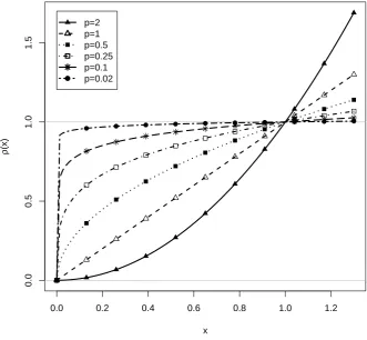
The statistical properties of the estimator forµandσalso strongly depend on the choice of the loss
0.0 0.2 0.4 0.6 0.8 1.0 1.2
0.0
0.5
1.0
1.5
x
ρ
(x
)
●
● ● ● ● ● ●
● ● ● ●
●
p=2 p=1 p=0.5 p=0.25 p=0.1 p=0.02
Figure 1.Lploss functionρ(x) =|x|pfor different values ofp.
The loss functionρ
(
x) =
|
x|
pis not differentiable forp≤
1 that prevent from using optimization algorithms that rely on derivatives. However, in the alignment, the function ρ is replaced by a differentiable approximating functionρD(
x) = (
x2+
ε)
p/2using a smallε>
0 (e.g.,ε=
.01 [used in the software Mplus] orε=
.001). BecauseρDis differentiable, quasi-Newton minimization approaches can be used that are implemented in standard optimizers in R [55]. In our experience, in the case of smallεvalues, the optimization of the alignment function is very sensitive to starting values [see also 4]. Hence, the implementation in the sirt [53] package specifies a sequence of decreasing values ofεin the optimization, each using the previous solution as initial values (see [56] for a similar approach).There are a few simulation studies that investigate the behavior of the IA method withp
=
0.5. Previous simulation studies for unidimensional factor model investigated the case of continuous items [4,31,57,58], dichotomous items [59,60], and polytomous items [61,62]. The extension of IA to multidimensional factor models with continuous items was discussed in [63] and [64]. As the IA approach is implemented in the popular Mplus software, it was already employed in a broad range of applications [34,64–83].3.2. Haberman Linking
TheHaberman linking(HL) approach [5] also has the goal of linking multiple groups. In contrast to the IA approach, HL also estimates joint item loadingsλ
= (
λ1, . . . ,λI)
and item difficultiesβ
= (
β1, . . . ,βI)
or item interceptsν= (
ν1, . . . ,νI)
. HL is conducted in two estimation steps. In the first step, the group standard deviationsσare computed. In the second step, the group meansµarecomputed. We now describe the estimation procedure in detail.
In the first step, estimated item loadings ˆλg (g
=
1, . . . ,G) are used to obtain group standard deviations σ and joint item loadingsλ by minimizing a criterionH1(
σ,λ)
. Using logarithmizedH1l
(
σ,λ) =
I
∑
i=1G
∑
g=1ρ log ˆλig,0
−
logλi−
logσg (19)Whereρis a loss function. In this article, the loss functionρ
(
x) =
|
x|
pis applied like for the IA method. Haberman [5] usedp=
2 forρin Equation19. Alternatively, one can employ untransformed item loadings for determiningσ andλ. In this case, untransformed estimated item loadings are used andone minimizes
H1u
(
σ,λ) =
I
∑
i=1G
∑
g=1ρ λˆig,0
−
λi−
σg (20)In the second step, estimated item interceptsνgand standard deviations ˆσgfrom the first step (g
=
1, . . . ,G) are used to compute group meansµand item difficultiesβ. By using Equation8, thefollowing criterion originally proposed by Haberman [5] is minimized
H2d
(
µ,β) =
I
∑
i=1G
∑
g=1ρ σˆg ˆ νig,0 ˆ λig,0
+
βig−
µg !(21)
Alternatively, one can use Equation4for motivating the minimization of the following linking function
H2i
(
µ,ν) =
I
∑
i=1G
∑
g=1ρ νˆig,0
−
νig−
ˆ λig,0ˆ σg µg
!
(22)
In this case, item interceptsνinstead of item difficultiesβare estimated.
As for the IA approach, the HL method can be applied by combining the two alternatives of minimization functionsH1uorH1l andH2norH2lfor standard deviations and means, respectively. Again, four different linking functions can be defined:H1uandH2i(Method HL1),H1landH2i(Method HL2),H1uandH2d(Method HL3), andH1landH2d(Method HL4). The originally proposed Haberman method is Method HL4 with the loss functionρ
(
x) =
x2(i.e.,p=
2).HL has been studied in [84] and is implemented in the R packages equateIRT [85] (function
multiec()) and sirt [53] (functionslinking.haberman()andlinking.haberman.lq()). SAS code is also
available [86]. The linking of multiple groups using other linking functions has been treated in [84,87–89]. In contrast to the IA method, HL has only been scarcely applied [90–98].
4. Simulation Studies
In this section, we present two simulations studies that compare different specifications of IA and HL. In Study 1 (Section4.1), we consider continuous items. In Study 2 (Section4.2), we investigate the case of dichotomous items.
4.1. Study 1: Continuous Items
4.1.1. Simulation Design
In the no DIF condition, all item parameters were assumed to be invariant across groups. In the DIF condition, we generated item responses so that in each group there is exactly one noninvariant item intercept and one noninvariant item loading. In all groups, the invariant loadings and the residual variances of the indicator variables were set toλi
=
1 (i=
1, . . . , 5)
and the invariant item intercepts of the were set toνi=
0. The noninvariant item parameters in the first group wereν51=
0.5 and λ13=
1.4. The noninvariant item parameters in the second group wereν12=
−0.5 and
λ52=
0.5. The noninvariant item parameters in the third group wereν23=
0.5 andλ43=
0.3. In the case of 6 groups, item parameters of Groupg+
hwere chosen to be equal to item parameters of Groupg(g=
1, 2, 3; h=
1, 2, 3). For each condition,R=
300 replications were used.4.1.2. Analysis Methods
The performance of IA and HL was investigated by varying specifications of the linking functions. Four IA and HL specifications were tested: IA1, IA2, IA3, and IA4 (see Sect.3.1), and HL1, HL2, HL3, and HL4 (see Sect.3.2). For IA and HL, the powersp
=
0.02, 0.01, 0.25, 0.50, 1, and 2 were used in the linking functions.To identify group means and group standard deviations in the linking procedure, for the first group, the mean was set to 0 and the standard deviation was set to 1. After estimating all group means and group standard deviations, these parameters were transformed to obtain a mean of 0 and a standard deviation 1 for the total sample comprising all groups. These conditions were also fulfilled in the data generating model.
The statistical performance of the vector of estimated means ˆµand estimated standard deviations
ˆ
σis assessed by summarizing bias and variability of estimators across groups. Letγ
= (
γ1, . . . ,γG)
be a parameter of interest and ˆγ= (
γ1ˆ , . . . , ˆγG)
its estimator (i.e., for means and standard deviations). ForRreplications, the obtained estimates are ˆγr= (
γˆ1r, . . . , ˆγGr)
(r=
1, . . . ,R)
. The average absolute bias (ABIAS) is defined asABI AS
(
γˆ) =
1 GG
∑
g=11 R R
∑
r=1 ˆ γgr−
γg
=
1 G G∑
g=1
Bias
(
γˆg)
(23)The average root mean square error (ARMSE) is computed as
ARMSE
(
γˆ) =
1 GG
∑
g=1v u u t1 R R
∑
r=1ˆ
γgr
−
γg2=
1 GG
∑
g=1RMSE
(
γˆg)
. (24)The ARMSE is the average of the root mean square error (RMSE) of each parameter estimate. In all analyses, the software R [55] was used. Haberman linking and invariance alignment was performed with the R package sirt [53].
4.1.3. Results
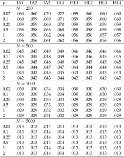
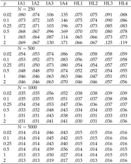
Table 1.Study 1: Average Root Mean Square Error (ARMSE) of Group Means as a Function of Sample Size in the Condition of No Differential Item Functioning (No DIF) andG=6 Groups
p IA1 IA2 IA3 IA4 HL1 HL2 HL3 HL4
N=250
0.02 .060 .060 .070 .072 .059 .060 .060 .060
0.1 .060 .059 .069 .071 .059 .059 .060 .060
0.25 .059 .059 .068 .070 .059 .059 .059 .059
0.5 .058 .058 .066 .068 .058 .058 .059 .058
1 .056 .056 .062 .064 .056 .056 .057 .057
2 .056 .056 .061 .062 .056 .056 .056 .056
N=500
0.02 .045 .045 .049 .049 .046 .046 .046 .046
0.1 .045 .045 .048 .049 .046 .046 .045 .045
0.25 .045 .045 .048 .048 .045 .045 .045 .045
0.5 .044 .044 .047 .047 .044 .044 .044 .044
1 .043 .043 .045 .045 .043 .043 .043 .043
2 .042 .042 .043 .044 .042 .042 .042 .042
N=1000
0.02 .030 .030 .034 .034 .030 .030 .030 .030
0.1 .030 .030 .034 .034 .030 .030 .030 .030
0.25 .030 .030 .033 .034 .029 .029 .029 .029
0.5 .029 .029 .033 .033 .029 .029 .029 .029
1 .029 .029 .032 .032 .029 .029 .029 .029
2 .029 .029 .031 .032 .029 .029 .029 .029
N=5000
0.02 .013 .013 .014 .014 .013 .013 .013 .013
0.1 .013 .013 .014 .014 .013 .013 .013 .013
0.25 .013 .013 .014 .014 .013 .013 .013 .013
0.5 .013 .013 .014 .014 .013 .013 .013 .013
1 .013 .013 .014 .014 .013 .013 .013 .013
2 .013 .013 .014 .014 .013 .013 .013 .013
Note. p= power used in invariance alignment (IA) or Haberman linking (HL) approaches; N =
sample size; IA1 corresponds to the IA specification proposed by Asparouhov and Muthén [4], and HL3 is the original specification of Haberman [5].
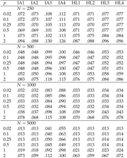
Table 2.Study 1: Average Root Mean Square Error (ARMSE) of Group Means as a Function of Sample Size in the Condition of Differential Item Functioning (DIF) andG=6 Groups
p IA1 IA2 IA3 IA4 HL1 HL2 HL3 HL4
N=250
0.02 .072 .073 .108 .112 .071 .071 .077 .077
0.1 .072 .073 .107 .111 .071 .071 .077 .077
0.25 .070 .070 .105 .113 .070 .070 .077 .077
0.5 .069 .069 .101 .108 .071 .071 .077 .077
1 .073 .071 .102 .113 .075 .075 .084 .084
2 .094 .088 .130 .126 .087 .088 .096 .096
N=500
0.02 .048 .048 .099 .100 .046 .046 .053 .053
0.1 .048 .048 .095 .098 .047 .047 .052 .052
0.25 .048 .048 .094 .097 .047 .047 .052 .052
0.5 .048 .048 .096 .100 .047 .047 .051 .051
1 .052 .050 .096 .108 .053 .053 .058 .059
2 .083 .075 .118 .115 .076 .075 .084 .086
N=1000
0.02 .032 .032 .083 .088 .033 .033 .034 .034
0.1 .032 .032 .085 .086 .033 .033 .034 .034
0.25 .033 .033 .084 .090 .033 .033 .033 .033
0.5 .032 .032 .084 .094 .032 .032 .034 .034
1 .038 .037 .098 .108 .039 .039 .043 .043
2 .078 .068 .115 .108 .070 .068 .076 .078
N=5000
0.02 .013 .013 .041 .055 .013 .013 .013 .013
0.1 .013 .013 .040 .063 .013 .013 .013 .014
0.25 .013 .013 .050 .066 .013 .013 .014 .014
0.5 .013 .013 .045 .049 .013 .013 .014 .014
1 .019 .018 .092 .098 .021 .021 .023 .024
2 .073 .059 .112 .100 .063 .059 .067 .072
Note. p= power used in invariance alignment (IA) or Haberman linking (HL) approaches; N =
sample size; IA1 corresponds to the IA specification proposed by Asparouhov and Muthén [4], and HL3 is the original specification of Haberman [5].
In Table2, the ARMSE is shown in the condition of DIF andG
=
6 groups. Alignment methods IA3 and IA4 that rely on linking item difficulties are inferior to all other methods, even for huge sample sizes. It can be seen that the methods (except IA3 and IA4) performed very similar for power values p=
0.02, 0.1, 0.25, and 0.5 for sample sizes of at least 500. Using a p of at least 0.5 is effective in reducing the bias introduced by linking usingp=
1 orp=
2. For a small sample size ofN=
250, p=
0.1 orp=
0.02 introduced non-negligible amounts of uncertainty. In general, the linking methods IA1, IA2, HL1, and HL2 have comparable performance. Notably, the additional number of estimated common item parameters in HL did not introduce additional variability in estimated group means. Moreover, it was found that HL based on item difficulties (as originally proposed in [5]; methods HL3 and HL4) resulted in more variable estimates than HL based on item difficulties (methods HL1 and HL2).The results for the ARMSE for 3 groups were almost identical to 6 groups, see Tables A5 and A6 in Supplement A.
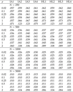
Table 3. Study 1: Average Root Mean Square Error (ARMSE) of Group Standard Deviations as a Function of Sample Size in the Condition of Differential Item Functioning (DIF) andG=6 Groups
p IA1 IA2 IA3 IA4 HL1 HL2 HL3 HL4
N=250
0.02 .057 .059 .062 .061 .062 .059 .062 .060
0.1 .057 .059 .061 .060 .061 .059 .062 .060
0.25 .056 .058 .061 .060 .061 .059 .062 .060
0.5 .055 .058 .060 .060 .062 .059 .062 .060
1 .057 .066 .067 .060 .073 .069 .073 .070
2 .071 .123 .123 .075 .107 .123 .107 .123
N=500
0.02 .036 .036 .041 .041 .037 .037 .037 .038
0.1 .036 .035 .040 .041 .037 .037 .037 .037
0.25 .035 .035 .040 .041 .036 .036 .037 .037
0.5 .035 .035 .039 .041 .036 .036 .036 .036
1 .037 .041 .043 .043 .045 .044 .045 .044
2 .060 .108 .106 .066 .089 .108 .089 .107
N=1000
0.02 .026 .026 .029 .030 .025 .025 .025 .026
0.1 .026 .025 .029 .030 .025 .025 .025 .025
0.25 .025 .025 .029 .030 .025 .025 .025 .025
0.5 .025 .025 .028 .030 .025 .025 .026 .026
1 .028 .032 .034 .034 .035 .035 .035 .035
2 .056 .106 .103 .061 .088 .106 .087 .105
N=5000
0.02 .010 .010 .013 .015 .010 .010 .010 .010
0.1 .010 .010 .013 .016 .010 .010 .010 .011
0.25 .010 .011 .014 .016 .010 .011 .011 .011
0.5 .011 .011 .013 .014 .011 .011 .011 .011
1 .013 .017 .020 .020 .020 .021 .019 .021
2 .050 .104 .098 .055 .086 .104 .084 .102
Note. p= power used in invariance alignment (IA) or Haberman linking (HL) approaches; N =
sample size; IA1 corresponds to the IA specification proposed by Asparouhov and Muthén [4], and HL3 is the original specification of Haberman [5].
In Table3, the ARMSE of group standard deviations for 6 groups in the DIF condition is shown. For power valuesp
=
0.02 top=
0.5, the methods IA1, IA2, HL1, and HL2 were similar, but provided substantially different results forp=
1 andp=
2.Overall, simulation study 1 showed that HL could be regarded to be very similar to IA by using the same robust loss function as in IA. Both approaches can be effectively used to reduce bias in estimated group distribution parameters in the situation of partial invariance.
4.2. Study 2: Dichotomous Items
4.2.1. Simulation Design
DIF effect. The item parameters were held constant across conditions and replications. In total,I
=
20 items were used in the simulation.For each item in each group and for a fixed proportionπBof items with DIF effects, a discrete variableZig, which had values of 0 (if the item had an invariant item intercept), or
+
1 (biased item with a uniform DIF effect). The constant DIF effectδwas chosen either 0 (no DIF condition), or 0.6 (DIF condition). All biased items within a group received a uniform DIF effect of either+
δor−
δ. This property was implemented by defining a variableDgthat had either a value of 1 or−1. The DIF
effects for unbalanced DIF were defined aseig=
ZigDgδ.For each condition of the simulation design,R
=
300 replications were generated. We manipulated the number of persons per group (N=
250, 500, 1000, and 5000). We fixed the proportion of items with DIF effects to 30% (i.e., in every group, 6 out of 20 items have DIF effects).4.2.2. Analysis Methods
The same four IA and HL methods were tested as in simulation study 1. Again, power values p
=
0.02, 0.1, 0.25, 0.5, 1, and 2 were compared. We implemented the IA and HL approaches in the sirt package [53] and used the TAM package [99] for estimating the 2PL model with marginal maximum likelihood.4.2.3. Results
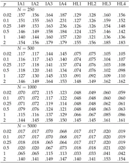
Table 4.Study 2: Average Root Mean Square Error (ARMSE) of Group Means as a Function of Sample Size in the Condition of No Differential Item Functioning (No DIF) andG=6 Groups
p IA1 IA2 IA3 IA4 HL1 HL2 HL3 HL4
N=250
0.02 .080 .074 .106 .135 .075 .075 .091 .088
0.1 .073 .072 .105 .146 .075 .074 .090 .086
0.25 .072 .071 .103 .196 .073 .073 .085 .083
0.5 .068 .067 .096 .169 .070 .070 .080 .078
1 .065 .064 .087 .114 .065 .066 .073 .073
2 .069 .067 .130 .171 .066 .067 .125 .119
N=500
0.02 .054 .053 .074 .086 .056 .058 .058 .059
0.1 .053 .052 .073 .083 .056 .057 .057 .058
0.25 .051 .050 .073 .080 .054 .054 .057 .057
0.5 .048 .048 .070 .074 .052 .052 .054 .055
1 .046 .046 .063 .063 .046 .047 .051 .051
2 .046 .046 .063 .070 .046 .046 .057 .056
N=1000
0.02 .035 .035 .056 .052 .038 .038 .039 .039
0.1 .035 .035 .055 .051 .037 .037 .038 .038
0.25 .034 .034 .053 .047 .036 .036 .037 .037
0.5 .033 .032 .048 .043 .034 .034 .035 .036
1 .031 .031 .043 .038 .031 .031 .033 .033
2 .031 .031 .041 .041 .030 .031 .036 .036
N=5000
0.02 .014 .014 .046 .043 .015 .015 .016 .016
0.1 .014 .014 .045 .042 .015 .015 .016 .016
0.25 .014 .014 .043 .040 .015 .014 .016 .016
0.5 .014 .014 .039 .036 .014 .014 .016 .015
1 .013 .013 .030 .027 .014 .014 .015 .015
2 .013 .013 .019 .017 .013 .013 .016 .016
Note. p= power used in invariance alignment (IA) or Haberman linking (HL) approaches; N =
In Table4, the ARMSE of the estimated group means is shown in the condition of no DIF and 6 groups. IA methods IA1 and IA2 performed slightly better than HL for a small powerp. Like for normally distributed item responses, using a powerpsmaller than 2 in the no DIF conditions results in some loss of efficiency in estimated group means. Moreover, methods IA3 and IA4 that perform alignment based on item difficulties were again clearly inferior to alignment based on item intercepts (methods IA1 and IA2). In Table B1 and B2 in Supplement B, the ABIAS is shown for 3 and 6 groups. The ARMSE in the case of 6 groups and the no DIF condition is shown in Table B5.
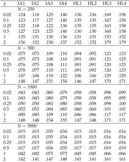
Table 5.Study 2: Average Root Mean Square Error (ARMSE) of Group Means as a Function of Sample Size in the Condition of Differential Item Functioning (DIF) andG=6 Groups
p IA1 IA2 IA3 IA4 HL1 HL2 HL3 HL4
N=250
0.02 .157 .156 .164 .187 .129 .128 .160 .156
0.1 .151 .155 .163 .231 .127 .126 .159 .152
0.25 .149 .153 .163 .236 .126 .126 .154 .148
0.5 .146 .149 .158 .184 .124 .125 .146 .142
1 .140 .144 .160 .157 .120 .121 .136 .136
2 .154 .156 .179 .179 .155 .156 .185 .183
N=500
0.02 .117 .117 .144 .145 .075 .075 .105 .105
0.1 .116 .117 .143 .140 .074 .075 .104 .107
0.25 .117 .118 .141 .137 .074 .076 .103 .108
0.5 .118 .120 .141 .134 .074 .076 .102 .098
1 .127 .130 .145 .133 .091 .092 .109 .110
2 .146 .149 .164 .153 .148 .149 .162 .162
N=1000
0.02 .070 .072 .115 .123 .048 .049 .060 .059
0.1 .071 .072 .117 .122 .048 .048 .060 .060
0.25 .071 .072 .119 .114 .048 .048 .062 .061
0.5 .079 .076 .124 .121 .048 .048 .063 .063
1 .115 .116 .137 .129 .066 .067 .085 .086
2 .144 .145 .158 .150 .145 .145 .161 .161
N=5000
0.02 .017 .017 .070 .068 .017 .017 .020 .019
0.1 .017 .017 .070 .068 .017 .017 .020 .019
0.25 .018 .018 .065 .064 .017 .017 .020 .019
0.5 .020 .020 .067 .073 .018 .018 .021 .020
1 .065 .065 .115 .113 .033 .033 .041 .042
2 .140 .141 .149 .147 .140 .141 .153 .154
Note. p= power used in invariance alignment (IA) or Haberman linking (HL) approaches; N =
sample size; IA1 corresponds to the IA specification proposed by Asparouhov and Muthén [4], and HL3 is the original specification of Haberman [5].
Table 6.Study 2: Average Root Mean Square Error (ARMSE) of Group Means as a Function of Sample Size in the Condition of Differential Item Functioning (DIF) andG=3 Groups
p IA1 IA2 IA3 IA4 HL1 HL2 HL3 HL4
N=250
0.02 .124 .118 .125 .140 .136 .136 .169 .158
0.1 .123 .117 .127 .140 .135 .135 .167 .158
0.25 .122 .118 .122 .136 .135 .135 .163 .158
0.5 .127 .123 .125 .140 .130 .130 .160 .158
1 .135 .131 .130 .136 .131 .131 .153 .152
2 .156 .152 .150 .157 .152 .152 .179 .179
N=500
0.02 .075 .073 .109 .110 .094 .092 .123 .123
0.1 .075 .073 .108 .110 .091 .091 .123 .125
0.25 .076 .075 .108 .111 .091 .091 .120 .125
0.5 .078 .077 .110 .111 .091 .092 .120 .123
1 .107 .106 .118 .122 .106 .106 .129 .129
2 .148 .147 .151 .154 .146 .147 .170 .171
N=1000
0.02 .043 .043 .080 .079 .058 .058 .098 .099
0.1 .043 .043 .080 .079 .058 .058 .095 .095
0.25 .050 .050 .082 .080 .058 .058 .098 .100
0.5 .052 .052 .084 .083 .060 .060 .101 .101
1 .085 .085 .109 .110 .086 .086 .117 .117
2 .148 .148 .154 .155 .147 .148 .171 .171
N=5000
0.02 .015 .015 .035 .034 .015 .015 .016 .016
0.1 .015 .015 .035 .034 .015 .015 .016 .016
0.25 .015 .015 .035 .034 .015 .015 .016 .016
0.5 .017 .017 .036 .035 .017 .017 .019 .019
1 .042 .042 .073 .073 .045 .045 .066 .066
2 .142 .141 .147 .148 .141 .141 .161 .161
Note. p= power used in invariance alignment (IA) or Haberman linking (HL) approaches; N =
sample size; IA1 corresponds to the IA specification proposed by Asparouhov and Muthén [4], and HL3 is the original specification of Haberman [5].
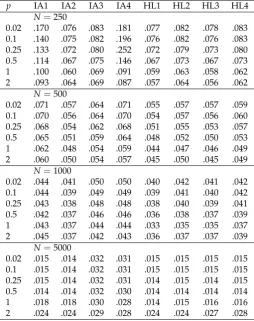
Table 7. Study 2: Average Root Mean Square Error (ARMSE) of Group Standard Deviations as a Function of Sample Size in the Condition of Differential Item Functioning (DIF) andG=6 Groups
p IA1 IA2 IA3 IA4 HL1 HL2 HL3 HL4
N=250
0.02 .170 .076 .083 .181 .077 .082 .078 .083
0.1 .140 .075 .082 .196 .076 .082 .076 .083
0.25 .133 .072 .080 .252 .072 .079 .073 .080
0.5 .114 .067 .075 .146 .067 .073 .067 .073
1 .100 .060 .069 .091 .059 .063 .058 .062
2 .093 .064 .069 .087 .057 .064 .056 .062
N=500
0.02 .071 .057 .064 .071 .055 .057 .057 .059
0.1 .070 .056 .064 .070 .054 .057 .056 .060
0.25 .068 .054 .062 .068 .051 .055 .053 .057
0.5 .065 .051 .059 .064 .048 .052 .050 .053
1 .062 .048 .054 .059 .044 .047 .046 .049
2 .060 .050 .054 .057 .045 .050 .045 .049
N=1000
0.02 .044 .041 .050 .050 .040 .042 .041 .042
0.1 .044 .039 .049 .049 .039 .041 .040 .042
0.25 .043 .038 .048 .048 .038 .040 .039 .041
0.5 .042 .037 .046 .046 .036 .038 .037 .039
1 .043 .037 .044 .044 .033 .035 .035 .037
2 .045 .037 .042 .043 .036 .037 .037 .039
N=5000
0.02 .015 .014 .032 .031 .015 .015 .015 .015
0.1 .015 .014 .032 .031 .015 .015 .015 .015
0.25 .015 .014 .032 .031 .014 .015 .014 .015
0.5 .014 .014 .032 .030 .014 .014 .014 .014
1 .018 .018 .030 .028 .014 .015 .016 .016
2 .024 .024 .029 .028 .024 .024 .027 .028
Note. p= power used in invariance alignment (IA) or Haberman linking (HL) approaches; N =
sample size; IA1 corresponds to the IA specification proposed by Asparouhov and Muthén [4], and HL3 is the original specification of Haberman [5].
Finally, in Table7, the ARMSE for estimated standard deviations forG
=
6 groups in the DIF condition is shown. It can be seen that alignment based on untransformed item loadings (IA1), as originally proposed in [4] had inferior performance compared to using logarithmized item loadings (IA2). Like for group means, estimated group standard deviations for HL resulted in more precise estimates than for IA.To conclude, simulation study 2 provided a mixed pattern of findings regarding the superiority of one method over the other. For a smaller number of groups (G
=
3), IA was preferable, while for a larger number of groups (G=
6), HL was preferable. For a sufficiently large sample (e.g.,N≥
500), power values smaller than the original proposal ofp=
0.5 (see [4]) provide smaller biases and more precise estimates.5. Empirical Example: 2PL Study
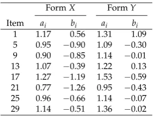
Table 8.2PL Study: Item Parameters Taken from Meyer and Zhou
FormX FormY
Item ai bi ai bi
1 1.17 0.56 1.31 1.09
5 0.95 −0.90 1.09 −0.30
9 0.90 −0.85 1.14 −0.01
13 1.07 −0.39 1.22 0.13
17 1.27 −1.19 1.53 −0.59
21 0.77 −1.26 0.95 −0.43
25 0.96 −0.66 1.14 −0.07
29 1.14 −0.51 1.36 −0.02
The original application was a linking study in which two test formsXandYshould be linked onto a common scale using 8 common items (displayed in Table8). The computation of linking constants is equivalent to the computation of group means and standard deviations in the case of two groups of persons that correspond to formsXandY. We estimated the mean and the standard deviation of the second group (i.e., FormY) while for the first group the mean was set to 0 and the standard deviation was set to 1. As in the simulation studies, we specified different variants of IA and HA as well as different power valuespin the loss function.
Table 9.2PL Study: Group Mean Corresponding to FormY
p IA1 IA2 IA3 IA4 HL1 HL2 HL3 HL4
0.02 −0.43 −0.43 −0.34 −0.34 −0.57 −0.57 −0.54 −0.54 0.1 −0.43 −0.43 −0.34 −0.34 −0.57 −0.57 −0.54 −0.54 0.25 −0.43 −0.43 −0.34 −0.34 −0.57 −0.57 −0.55 −0.55 0.5 −0.44 −0.44 −0.35 −0.35 −0.57 −0.57 −0.55 −0.55
1 −0.47 −0.47 −0.44 −0.44 −0.58 −0.58 −0.58 −0.58
2 −0.60 −0.60 −0.62 −0.62 −0.59 −0.59 −0.62 −0.62
Note. p= power used in invariance alignment (IA) or Haberman linking (HL) approaches; N =
sample size; IA1 corresponds to the IA specification proposed by Asparouhov and Muthén [4], and HL3 is the original specification of Haberman [5].
In Table9, the obtained means for the second group are displayed. It turned out that all Haberman approaches (HL) led to similar results, relatively independent of the choicep. Interestingly, IA and HL only resulted in similar estimates of the mean forp
=
2. Forp≤
1, IA produced substantially lower group differences (in terms of absolute values). The IA approaches based on item difficulties (IA3 and IA4) was different from the use of item intercepts (IA1 and IA2). However, no substantial differences for logarithmized and untransformed item loadings were obtained. Overall, this example shows that the use of a particular linking method can affect the outcomes of group comparisons.6. Discussion
In this article, we investigated the performance of extensions of invariance alignment (IA; [4]) and Haberman linking (HL; [5]) with respect to the flexibility of linking function in the analysis of more than two groups. The linking functions build on the principle that deviations between group-specific item parameters should be made as small and as sparse as possible. We have proposed a class of linking functions based on the family of robustLploss functionsρ
(
x) =
|
x|
p(p≥
0). It was shown that using robust link functions in HL can have similar performance to IA.As it is true for all simulation studies, our study has some limitations. First, we restricted the number of groups to at most 6. For international large-scale assessments like PISA (e.g., [101]), the number of groups–countries in this case–are much larger, say 30, or even 50. As IA was mostly advertised for applications involving many groups [31], it would be interesting whether robust HL would be competitive in this situation. Second, we only used 5 continuous items and 20 dichotomous items in the simulation studies. The performance of the linking methods with an increasing number of items could be a relevant topic future research (see [54]). Third, we restricted ourselves to dichotomous data. The performance of IA and HL for polytomous items (see [62]) or the mixed case of dichotomous and polytomous items could be investigated in future studies.
In the simulation study and the empirical example, different values of the powerpof the loss function were compared. It should be noted that using a particular type of loss functions can be reinterpreted as an optimal estimation method that corresponds to some distributional assumption of deviations between group-specific item parameters. By using this idea, the powerpin the loss function can be estimated by means of the exponential power distribution [102,103]; see [104] for a two-step estimation algorithm.
The choice of a particular value of the powerpin the linking function implies a decision whether some items (or item parameters) should be treated as outliers in a group comparison [94]. Typically, outliers are down-weighted in the estimation. Hence, the group-specific contribution of items to a group mean is determined by a statistical approach. In contrast, usingp
=
2 corresponds to a quadratic loss function, and all items contribute to the computation of group means. Several researchers have argued that the decision to eliminate items from group comparisons should be (mainly) driven by substantive considerations (see [94,105–110]).The presence of DIF effects introduces an additional source of ambiguity in determining group means in latent variable models. A consequence of noninvariance is that a subset of items can provide different group means even for infinite sample sizes. In large-scale assessment studies, this source of uncertainty that is due to a selection of a particular set of items has been labeled as linking errors [111–118]. Uncertainty in group means due to item sampling has also been extensively studied in generalizability theory [119–121].
Funding:This research received no external funding.
Conflicts of Interest:The authors declare no conflict of interest.
Abbreviations
The following abbreviations are used in this manuscript:
2PL two-parameter logistic model ABIAS average absolute bias
ARMSE average root mean square error DIF differential item functioning
HL Haberman linking
IA invariance alignment
PISA programme for international student assessment RMSE root mean square error
References
1. Mellenbergh, G.J. Item bias and item response theory. Int. J. Educ. Res. 1989, 13, 127–143. doi:10.1016/0883-0355(89)90002-5.
2. Millsap, R.E.Statistical approaches to measurement invariance; Routledge: New York, 2012.
3. van de Vijver, F.J.R., Ed. Invariance analyses in large-scale studies; OECD: Paris, 2019. doi:10.1787/254738dd-en.
4. Asparouhov, T.; Muthén, B. Multiple-group factor analysis alignment. Struct. Equ. Modeling2014,
21, 495–508. doi:10.1080/10705511.2014.919210.
5. Haberman, S.J. Linking parameter estimates derived from an item response model through separate calibrations
(Research Report No. RR-09-40). Educational Testing Service, 2009. doi:10.1002/j.2333-8504.2009.tb02197.x. 6. McDonald, R.P.Test theory: A unified treatment; Lawrence Erlbaum Associates Publishers, 1999.
7. Birnbaum, A. Some latent trait models and their use in inferring an examinee’s ability. InStatistical theories
of mental test scores; Lord, F.M.; Novick, M.R., Eds.; MIT Press: Reading, MA, 1968; pp. 397–479.
8. van der Linden, W.J.; Hambleton, R.K., Eds. Handbook of modern item response theory; 1997. doi:10.1007/978-1-4757-2691-6.
9. Yen, W.M.; Fitzpatrick, A.R. Item response theory. InEducational measurement; Brennan, R.L., Ed.; Praeger Publishers, 2006; pp. 111–154.
10. Meredith, W. Measurement invariance, factor analysis and factorial invariance. Psychometrika1993,
58, 525–543. doi:10.1007/BF02294825.
11. Shealy, R.; Stout, W. A model-based standardization approach that separates true bias/DIF from group ability differences and detects test bias/DTF as well as item bias/DIF. Psychometrika1993,58, 159–194. doi:10.1007/BF02294572.
12. Byrne, B.M. Adaptation of assessment scales in cross-national research: Issues, guidelines, and caveats.
Int. Perspect. Psychol.2016,5, 51–65. doi:10.1037/ipp0000042.
13. Byrne, B.M.; Shavelson, R.J.; Muthén, B. Testing for the equivalence of factor covariance and mean structures: the issue of partial measurement invariance. Psychol. Bull. 1989, 105, 456–466. doi:10.1037/0033-2909.105.3.456.
14. von Davier, M.; Yamamoto, K.; Shin, H.J.; Chen, H.; Khorramdel, L.; Weeks, J.; Davis, S.; Kong, N.; Kandathil, M. Evaluating item response theory linking and model fit for data from PISA 2000–2012.Assess.
Educ.2019,26, 466–488. doi:10.1080/0969594X.2019.1586642.
15. Penfield, R.D.; Camilli, G. Differential item functioning and item bias. InHandbook of statistics, Vol. 26:
Psychometrics; Rao, C.R.; Sinharay, S., Eds.; 2007; pp. 125–167. doi:10.1016/S0169-7161(06)26005-X.
16. Dong, Y.; Dumas, D. Are personality measures valid for different populations? A systematic review of measurement invariance across cultures, gender, and age. Pers. Individ. Differ. 2020,160, 109956. doi:10.1016/j.paid.2020.109956.
17. Fischer, R.; Karl, J.A. A primer to (cross-cultural) multi-group invariance testing possibilities in R.Front.
18. Han, K.; Colarelli, S.M.; Weed, N.C. Methodological and statistical advances in the consideration of cultural diversity in assessment: A critical review of group classification and measurement invariance testing.
Psychol. Assess.2019,31, 1481–1496. doi:10.1037/pas0000731.
19. Svetina, D.; Rutkowski, L.; Rutkowski, D. Multiple-group invariance with categorical outcomes using updated guidelines: An illustration using Mplus and the lavaan/semtools packages.Struct. Equ. Modeling
2020,27, 111–130. doi:10.1080/10705511.2019.1602776.
20. van de Schoot, R.; Schmidt, P.; De Beuckelaer, A.; Lek, K.; Zondervan-Zwijnenburg, M. Editorial: Measurement invariance.Front. Psychol.2015,6, 1064. doi:10.3389/fpsyg.2015.01064.
21. Muthén, B.; Asparouhov, T. IRT studies of many groups: The alignment method. Front. Psychol.2014,
5, 978. doi:10.3389/fpsyg.2014.00978.
22. Zieger, L.; Sims, S.; Jerrim, J. Comparing teachers’ job satisfaction across countries: A multiple-pairwise measurement invariance approach. Educ. Meas.2019,38, 75–85. doi:10.1111/emip.12254.
23. von Davier, M.; von Davier, A.A. A unified approach to IRT scale linking and scale transformations.
Methodology2007,3, 115–124. doi:10.1027/1614-2241.3.3.115.
24. González, J.; Wiberg, M. Applying test equating methods: Using R; Springer: New York, 2017. doi:10.1007/978-3-319-51824-4.
25. Kolen, M.J.; Brennan, R.L. Test equating, scaling, and linking; Springer: New York, 2014. doi:10.1007/978-1-4939-0317-7.
26. Lee, W.C.; Lee, G. IRT linking and equating. InThe Wiley handbook of psychometric testing: A multidisciplinary
reference on survey, scale and test; Irwing, P.; Booth, T.; Hughes, D.J., Eds.; Wiley: New York, 2018; pp.
639–673. doi:10.1002/9781118489772.ch21.
27. Sansivieri, V.; Wiberg, M.; Matteucci, M. A review of test equating methods with a special focus on IRT-based approaches. Statistica2017,77, 329–352. doi:10.6092/issn.1973-2201/7066.
28. von Davier, A.A.; Carstensen, C.H.; von Davier, M. Linking competencies in horizontal, vertical, and longitudinal settings and measuring growth. InAssessment of competencies in educational contexts; Hartig, J.; Klieme, E.; Leutner, D., Eds.; Hogrefe: Göttingen, 2008; pp. 121–149.
29. Fox, J.P.; Verhagen, A.J. Random item effects modeling for cross-national survey data. InCross-cultural
analysis: Methods and applications; Davidov, E.; Schmidt, P.; Billiet, J., Eds.; Routledge: London, 2010; pp.
461–482.
30. Muthén, B.; Asparouhov, T. Bayesian structural equation modeling: A more flexible representation of substantive theory. Psychol. Methods2012,17, 313–335. doi:10.1037/a0026802.
31. Muthén, B.; Asparouhov, T. Recent methods for the study of measurement invariance with many groups: Alignment and random effects.Sociol. Methods Res.2018,47, 637–664. doi:10.1177/0049124117701488. 32. van de Schoot, R.; Kluytmans, A.; Tummers, L.; Lugtig, P.; Hox, J.; Muthén, B. Facing off with scylla
and charybdis: A comparison of scalar, partial, and the novel possibility of approximate measurement invariance.Front. Psychol.2013,4, 770. doi:10.3389/fpsyg.2013.00770.
33. Boer, D.; Hanke, K.; He, J. On detecting systematic measurement error in cross-cultural research: A review and critical reflection on equivalence and invariance tests. J. Cross-Cult. Psychol.2018,49, 713–734. doi:10.1177/0022022117749042.
34. Davidov, E.; Meuleman, B. Measurement invariance analysis using multiple group confirmatory factor analysis and alignment optimisation. InInvariance analyses in large-scale studies; van de Vijver, F.J.R., Ed.; OECD: Paris, 2019; pp. 13–20. doi:10.1787/254738dd-en.
35. Winter, S.D.; Depaoli, S. An illustration of Bayesian approximate measurement invariance with longitudinal data and a small sample size. Int. J. Behav. Dev. 2019. Advance online publication, doi:10.1177/0165025419880610.
36. Avvisati, F.; Le Donné, N.; Paccagnella, M. A meeting report: Cross-cultural comparability of questionnaire measures in large-scale international surveys. Meas. Instrum. Soc. Sci. 2019, 1, 8. doi:10.1186/s42409-019-0010-z.
37. Fox, J.Applied regression analysis and generalized linear models; Sage: Thousand Oaks, 2016.
38. De Boeck, P. Random item IRT models.Psychometrika2008,73, 533–559. doi:10.1007/s11336-008-9092-x. 39. Frederickx, S.; Tuerlinckx, F.; De Boeck, P.; Magis, D. RIM: A random item mixture model to detect
40. He, Y.; Cui, Z. Evaluating robust scale transformation methods with multiple outlying common items under IRT true score equating. Appl. Psychol. Meas.2020,44, 296–310. doi:10.1177/0146621619886050. 41. He, Y.; Cui, Z.; Fang, Y.; Chen, H. Using a linear regression method to detect outliers in IRT common item
equating.Appl. Psychol. Meas.2013,37, 522–540. doi:10.1177/0146621613483207.
42. He, Y.; Cui, Z.; Osterlind, S.J. New robust scale transformation methods in the presence of outlying common items. Appl. Psychol. Meas.2015,39, 613–626. doi:10.1177/0146621615587003.
43. Huynh, H.; Meyer, P. Use of robustzin detecting unstable items in item response theory models.Pract.
Assess. Res. Evaluation2010,15, 2. doi:10.7275/ycx6-e864.
44. Magis, D.; De Boeck, P. Identification of differential item functioning in multiple-group settings: A multivariate outlier detection approach. Multivar. Behav. Res. 2011, 46, 733–755. doi:10.1080/00273171.2011.606757.
45. Magis, D.; De Boeck, P. A robust outlier approach to prevent type I error inflation in differential item functioning. Educ. Psychol. Meas.2012,72, 291–311. doi:10.1177/0013164411416975.
46. Soares, T.M.; Gonçalves, F.B.; Gamerman, D. An integrated Bayesian model for DIF analysis.J. Educ. Behav.
Stat.2009,34, 348–377. doi:10.3102/1076998609332752.
47. Muthén, L.; Muthén, B.Mplus user’s guide. Eighth edition., 1998–2020. Los Angeles, CA: Muthén & Muthén. 48. Harvey, A.C. On the unbiasedness of robust regression estimators. Commun. Stat. – Theory Methods1978,
7, 779–783. doi:10.1080/03610927808827668.
49. Lipovetsky, S. OptimalLp-metric for minimizing powered deviations in regression. J. Mod. Appl. Stat.
Methods2007,6, 20. doi:10.22237/jmasm/1177993140.
50. Livadiotis, G. General fitting methods based onLqnorms and their optimization. Stats2020,3, 16–31. doi:10.3390/stats3010002.
51. Ramsay, J.O. A comparative study of several robust estimates of slope, intercept, and scale in linear regression. J. Am. Stat. Assoc.1977,72, 608–615.
52. Sposito, V.A. On unbiasedLpregression estimators. J. Am. Stat. Assoc.1982,77, 652–653.
53. Robitzsch, A. sirt: Supplementary item response theory models, 2020. R package version 3.9-4. https://CRAN.R-project.org/package=sirt.
54. Pokropek, A.; Lüdtke, O.; Robitzsch, A. An extension of the invariance alignment method for scale linking.
Psych. Test Assess. Model.2020,62, 303–334.
55. R Core Team. R: A language and environment for statistical computing, 2020. Vienna, Austria. https://www.R-project.org/.
56. Battauz, M. Regularized estimation of the nominal response model.Multivar. Behav. Res.2019. Advance online publication, doi:10.1080/00273171.2019.1681252.
57. Kim, E.S.; Cao, C.; Wang, Y.; Nguyen, D.T. Measurement invariance testing with many groups: A comparison of five approaches. Struct. Equ. Modeling 2017, 24, 524–544. doi:10.1080/10705511.2017.1304822.
58. Pokropek, A.; Davidov, E.; Schmidt, P. A Monte Carlo simulation study to assess the appropriateness of traditional and newer approaches to test for measurement invariance. Struct. Equ. Modeling2019,
26, 724–744. doi:10.1080/10705511.2018.1561293.
59. DeMars, C.E. Alignment as an alternative to anchor purification in DIF analyses. Struct. Equ. Modeling
2020,27, 56–72. doi:10.1080/10705511.2019.1617151.
60. Finch, W.H. Detection of differential item functioning for more than two groups: A Monte Carlo comparison of methods. Appl. Meas. Educ.2016,29, 30–45. doi:10.1080/08957347.2015.1102916.
61. Flake, J.K.; McCoach, D.B. An investigation of the alignment method with polytomous indicators under conditions of partial measurement invariance. Struct. Equ. Modeling 2018, 25, 56–70. doi:10.1080/10705511.2017.1374187.
62. Mansolf, M.; Vreeker, A.; Reise, S.P.; Freimer, N.B.; Glahn, D.C.; Gur, R.E.; Moore, T.M.; Pato, C.N.; Pato, M.T.; Palotie, A.; others. Extensions of multiple-group item response theory alignment: Application to psychiatric phenotypes in an international genomics consortium. Educ. Psychol. Meas.2020. Advance online publication, doi:10.1177/0013164419897307.
64. Marsh, H.W.; Guo, J.; Parker, P.D.; Nagengast, B.; Asparouhov, T.; Muthén, B.; Dicke, T. What to do when scalar invariance fails: The extended alignment method for multi-group factor analysis comparison of latent means across many groups. Psychol. Methods2018,23, 524–545. doi:10.1037/met0000113.
65. Borgonovi, F.; Pokropek, A. Can we rely on trust in science to beat the COVID-19 pandemic? PsyArXiv
2020. doi:10.31234/osf.io/yq287.
66. Brook, C.A.; Schmidt, L.A. Lifespan trends in sociability: Measurement invariance and mean-level differences in ages 3 to 86 years. Pers. Individ. Differ.2020,152, 109579. doi:10.1016/j.paid.2019.109579. 67. Coromina, L.; Bartolomé Peral, E. Comparing alignment and multiple group CFA for analysing political
trust in Europe during the crisis. Methodology2020,16, 21–40. doi:10.5964/meth.2791.
68. Davidov, E.; Cieciuch, J.; Meuleman, B.; Schmidt, P.; Algesheimer, R.; Hausherr, M. The comparability of measurements of attitudes toward immigration in the European Social Survey: Exact versus approximate measurement equivalence.Public Opin. Q.2015,79, 244–266. doi:10.1093/poq/nfv008.
69. De Bondt, N.; Van Petegem, P. Psychometric evaluation of the overexcitability questionnaire-two: Applying Bayesian structural equation modeling (BSEM) and multiple-group BSEM-based alignment with approximate measurement invariance. Front. Psychol.2015,6, 1963. doi:10.3389/fpsyg.2015.01963. 70. Fischer, J.; Praetorius, A.K.; Klieme, E. The impact of linguistic similarity on cross-cultural comparability
of students’ perceptions of teaching quality. Educ. Assess. Evaluation Account. 2019, 31, 201–220. doi:10.1007/s11092-019-09295-7.
71. Goel, A.; Gross, A. Differential item functioning in the cognitive screener used in the longitudinal aging study in India. Int. Psychogeriatr.2019,31, 1331–1341. doi:10.1017/S1041610218001746.
72. Jang, S.; Kim, E.S.; Cao, C.; Allen, T.D.; Cooper, C.L.; Lapierre, L.M.; O’Driscoll, M.P.; Sanchez, J.I.; Spector, P.E.; Poelmans, S.A.Y.; others. Measurement invariance of the satisfaction with life scale across 26 countries.
J. Cross-Cult. Psychol.2017,48, 560–576. doi:10.1177/0022022117697844.
73. Lek, K.; van de Schoot, R. Bayesian approximate measurement invariance. InInvariance analyses in
large-scale studies; van de Vijver, F.J.R., Ed.; OECD: Paris, 2019; pp. 21–35. doi:10.1787/254738dd-en.
74. Lomazzi, V. Using alignment optimization to test the measurement invariance of gender role attitudes in 59 countries. Methods Data Anal.2018,12, 77–103. doi:10.12758/mda.2017.09.
75. McLarnon, M.J.W.; Romero, E.F. Cross-cultural equivalence of shortened versions of the Eysenck personality questionnaire: An application of the alignment method. Pers. Individ. Differ.2020,163, 110074. doi:10.1016/j.paid.2020.110074.
76. Milfont, T.L.; Bain, P.G.; Kashima, Y.; Corral-Verdugo, V.; Pasquali, C.; Johansson, L.O.; Guan, Y.; Gouveia, V.V.; Garðarsdóttir, R.B.; Doron, G.; others. On the relation between social dominance orientation and environmentalism: A 25-nation study. Soc. Psychol. Pers. Sci. 2018, 9, 802–814. doi:10.1177/1948550617722832.
77. Munck, I.; Barber, C.; Torney-Purta, J. Measurement invariance in comparing attitudes toward immigrants among youth across Europe in 1999 and 2009: The alignment method applied to IEA CIVED and ICCS.
Sociol. Methods Res.2018,47, 687–728. doi:10.1177/0049124117729691.
78. Rescorla, L.A.; Adams, A.; Ivanova, M.Y. The CBCL/11/2–5’s DSM-ASD scale: Confirmatory factor analyses across 24 societies. J. Autism Dev. Disord. 2019. Advance online publication, doi:10.1007/s10803-019-04189-5.
79. Rice, K.G.; Park, H.J.; Hong, J.; Lee, D.g. Measurement and implications of perfectionism in South Korea and the United States. Couns. Psychol.2019,47, 384–416. doi:10.1177/0011000019870308.
80. Roberson, N.D.; Zumbo, B.D. Migration background in PISA’s measure of social belonging: Using a diffractive lens to interpret multi-method DIF studies. Int. J. Test. 2019, 19, 363–389. doi:10.1080/15305058.2019.1632316.
81. Seddig, D.; Leitgöb, H. Approximate measurement invariance and longitudinal confirmatory factor analysis: Concept and application with panel data. Surv. Res. Methods 2018, 12, 29–41. doi:10.18148/srm/2018.v12i1.7210.
83. Wickham, R.E.; Gutierrez, R.; Giordano, B.L.; Rostosky, S.S.; Riggle, E.D.B. Gender and generational differences in the internalized homophobia questionnaire: An alignment IRT analysis. Assessment2019. Advance online publication, doi:10.1177/1073191119893010.
84. Battauz, M. Multiple equating of separate IRT calibrations. Psychometrika 2017, 82, 610–636. doi:10.1007/s11336-016-9517-x.
85. Battauz, M. equateMultiple: Equating of multiple forms, 2017. R package version 0.0.0. https://CRAN.R-project.org/package=equateMultiple.
86. Yao, L.; Haberman, S.J.; Xu, J. Using SAS to implement simultaneous linking in item response theory, 2015. Technical report.
87. Arai, S.; Mayekawa, S.i. A comparison of equating methods and linking designs for developing an item pool under item response theory.Behaviormetrika2011,38, 1–16. doi:10.2333/bhmk.38.1.
88. Kang, H.A.; Lu, Y.; Chang, H.H. IRT item parameter scaling for developing new item pools.Appl. Meas.
Educ.2017,30, 1–15. doi:10.1080/08957347.2016.1243537.
89. Weeks, J.P. plink: An R package for linking mixed-format tests using IRT-based methods. J. Stat. Softw.
2010,35, 1–33. doi:10.18637/jss.v035.i12.
90. Becker, B.; Weirich, S.; Mahler, N.; Sachse, K.A. Testdesign und Auswertung des IQB-Bildungstrends 2018: Technische Grundlagen [Test design and analysis of the IQB education trend 2018: Technical foundations].
InIQB-Bildungstrend 2018. Mathematische und naturwissenschaftliche Kompetenzen am Ende der Sekundarstufe I
im zweiten Ländervergleich; Stanat, P.; Schipolowski, S.; Mahler, N.; Weirich, S.; Henschel, S., Eds.; Waxmann:
Münster, 2019; pp. 411–425.
91. Höft, L.; Bernholt, S. Longitudinal couplings between interest and conceptual understanding in secondary school chemistry: An activity-based perspective. Int. J. Sci. Educ. 2019, 41, 607–627. doi:10.1080/09500693.2019.1571650.
92. Moehring, A.; Schroeders, U.; Wilhelm, O. Knowledge is power for medical assistants: Crystallized and fluid intelligence as predictors of vocational knowledge. Front. Psychol. 2018, 9, 28. doi:10.3389/fpsyg.2018.00028.
93. Petrakova, A.; Sommer, W.; Junge, M.; Hildebrandt, A. Configural face perception in childhood and adolescence: An individual differences approach. Acta Psychol. 2018, 188, 148–176. doi:10.1016/j.actpsy.2018.06.005.
94. Robitzsch, A.; Lüdtke, O. A review of different scaling approaches under full invariance, partial invariance, and noninvariance for cross-sectional country comparisons in large-scale assessments.Psych. Test Assess.
Model.2020,62, 233–279.
95. Robitzsch, A.; Lüdtke, O.; Goldhammer, F.; Kroehne, U.; Köller, O. Reanalysis of the German PISA data: A comparison of different approaches for trend estimation with a particular emphasis on mode effects. Front.
Psychol.2020,11, 884. doi:10.3389/fpsyg.2020.00884.
96. Rösselet, S.; Neuenschwander, M.P. Akzeptanz und Ablehnung beim Übertritt in die Sekundarstufe I [Acceptance and rejection on tracking to lower secondary education]. InBildungsverläufe von der Einschulung
bis in den ersten Arbeitsmarkt; Neuenschwander, M.P.; Nägele, C., Eds.; Springer VS, 2017; pp. 103–121.
doi:10.1007/978-3-658-16981-7_6.
97. Sewasew, D.; Schroeders, U.; Schiefer, I.M.; Weirich, S.; Artelt, C. Development of sex differences in math achievement, self-concept, and interest from grade 5 to 7. Contemp. Educ. Psychol.2018,54, 55–65. doi:10.1016/j.cedpsych.2018.05.003.
98. Trendtel, M.; Pham, H.G.; Yanagida, T. Skalierung und Linking [Scaling and linking]. InLarge-Scale
Assessment mit R: Methodische Grundlagen der österreichischen Bildungsstandards-Überprüfung; Breit, S.;
Schreiner, C., Eds.; Facultas: Wien, 2016; pp. 185–224.
99. Robitzsch, A.; Kiefer, T.; Wu, M. TAM: Test analysis modules, 2020. R package version 3.4-26. https://CRAN.R-project.org/package=TAM.
100. Meyer, J.P.; Zhu, S. Fair and equitable measurement of student learning in MOOCs: An introduction to item response theory, scale linking, and score equating. Res. Pract. Assess.2013,8, 26–39.
101. OECD.PISA 2006. Technical report; OECD: Paris, 2009.
102. Mineo, A.M. On the estimation of the structure parameter of a normal distribution of orderp. Statistica
103. Mineo, A.M.; Ruggieri, M. A software tool for the exponential power distribution: The normalp package.
J. Stat. Softw.2005,12, 1–24. doi:10.18637/jss.v012.i04.
104. Giacalone, M.; Panarello, D.; Mattera, R. Multicollinearity in regression: An efficiency comparison between
Lp-norm and least squares estimators.Qual. Quant.2018,52, 1831–1859. doi:10.1007/s11135-017-0571-y. 105. Camilli, G. The case against item bias detection techniques based on internal criteria: Do item bias procedures obscure test fairness issues? InDifferential item functioning: Theory and practice; Holland, P.W.; Wainer, H., Eds.; Erlbaum: Hillsdale, NJ, 1993; pp. 397–417.
106. El Masri, Y.H.; Andrich, D. The trade-off between model fit, invariance, and validity: The case of PISA science assessments. Appl. Meas. Educ.2020,33, 174–188. doi:10.1080/08957347.2020.1732384.
107. Huang, X.; Wilson, M.; Wang, L. Exploring plausible causes of differential item functioning in the PISA science assessment: Language, curriculum or culture. Educ. Psychol. 2016, 36, 378–390. doi:10.1080/01443410.2014.946890.
108. Kuha, J.; Moustaki, I. Nonequivalence of measurement in latent variable modeling of multigroup data: A sensitivity analysis. Psychol. Methods2015,20, 523–536. doi:10.1037/met0000031.
109. Taherbhai, H.; Seo, D. The philosophical aspects of IRT equating: Modeling drift to evaluate cohort growth in large-scale assessments. Educ. Meas.2013,32, 2–14. doi:10.1111/emip.12000.
110. Zwitser, R.J.; Glaser, S.S.F.; Maris, G. Monitoring countries in a changing world: A new look at DIF in international surveys.Psychometrika2017,82, 210–232. doi:10.1007/s11336-016-9543-8.
111. Gebhardt, E.; Adams, R.J. The influence of equating methodology on reported trends in PISA. J. Appl.
Meas.2007,8, 305–322.
112. Michaelides, M.P. A review of the effects on IRT item parameter estimates with a focus on misbehaving common items in test equating. Front. Psychol.2010,1, 167. doi:10.3389/fpsyg.2010.00167.
113. Monseur, C.; Berezner, A. The computation of equating errors in international surveys in education. J.
Appl. Meas.2007,8, 323–335.
114. Monseur, C.; Sibberns, H.; Hastedt, D. Linking errors in trend estimation for international surveys in education. IERI Monogr. Ser.2008,1, 113–122.
115. Robitzsch, A.; Lüdtke, O. Linking errors in international large-scale assessments: Calculation of standard errors for trend estimation. Assess. Educ.2019,26, 444–465. doi:10.1080/0969594X.2018.1433633.
116. Sachse, K.A.; Roppelt, A.; Haag, N. A comparison of linking methods for estimating national trends in international comparative large-scale assessments in the presence of cross-national DIF. J. Educ. Meas.
2016,53, 152–171. doi:10.1111/jedm.12106.
117. Wu, M. Measurement, sampling, and equating errors in large-scale assessments. Educ. Meas. 2010,
29, 15–27. doi:10.1111/j.1745-3992.2010.00190.x.
118. Xu, X.; von Davier, M.Linking errors in trend estimation in large-scale surveys: A case study.(Research Report No. RR-10-10). Educational Testing Service, 2010. doi:10.1002/j.2333-8504.2010.tb02217.x.
119. Brennan, R.L. Generalizability theory.Educ. Meas.1992,11, 27–34. doi:10.1111/j.1745-3992.1992.tb00260.x. 120. Brennan, R.L.Generalizabilty theory; Springer: New York, 2001. doi:10.1007/978-1-4757-3456-0.
121. Cronbach, L.J.; Rajaratnam, N.; Gleser, G.C. Theory of generalizability: A liberalization of reliability theory.
Brit. J. Stat. Psychol.1963,16, 137–163. doi:10.1111/j.2044-8317.1963.tb00206.x.
122. Hastie, T.; Tibshirani, R.; Wainwright, M.Statistical learning with sparsity: The lasso and generalizations; CRC Press: Boca Raton, 2015. doi:10.1201/b18401.
123. Belzak, W.; Bauer, D.J. Improving the assessment of measurement invariance: Using regularization to select anchor items and identify differential item functioning. Psychol. Methods2020. Advance online publication, doi:10.1037/met0000253.
124. Huang, P.H. A penalized likelihood method for multi-group structural equation modelling. Brit. J. Math.
Stat. Psychol.2018,71, 499–522. doi:10.1111/bmsp.12130.
125. Liang, X.; Jacobucci, R. Regularized structural equation modeling to detect measurement bias: Evaluation of lasso, adaptive lasso, and elastic net. Struct. Equ. Modeling2019. Advance online publication, doi:10.1080/10705511.2019.1693273.
126. Schauberger, G.; Mair, P. A regularization approach for the detection of differential item functioning in generalized partial credit models. Behav. Res. Methods2020,52, 279–294. doi:10.3758/s13428-019-01224-2. 127. Tutz, G.; Schauberger, G. A penalty approach to differential item functioning in Rasch models.Psychometrika
128. Xu, Z.; Chang, X.; Xu, F.; Zhang, H. L1/2regularization: A thresholding representation theory and a fast solver.IEEE T. Neur. Net. Lear.2012,23, 1013–1027. doi:10.1109/TNNLS.2012.2197412.
129. Hu, Y.; Li, C.; Meng, K.; Qin, J.; Yang, X. Group sparse optimization vialp,qregularization. J. Mach. Learn.
Res.2017,18, 960–1011.
130. Wang, B.; Wan, W.; Wang, Y.; Ma, W.; Zhang, L.; Li, J.; Zhou, Z.; Zhao, H.; Gao, F. AnLp(0≤p≤1)-norm regularized image reconstruction scheme for breast DOT with non-negative-constraint. Biomed. Eng.