This content has been downloaded from IOPscience. Please scroll down to see the full text.
Download details:
IP Address: 195.195.217.51
This content was downloaded on 14/06/2016 at 15:48
Please note that terms and conditions apply.
The effect of aspect ratio on the leading-edge vortex over an insect-like flapping wing
View the table of contents for this issue, or go to the journal homepage for more 2015 Bioinspir. Biomim. 10 056020
PAPER
The effect of aspect ratio on the leading-edge vortex over an
insect-like
fl
apping wing
Nathan Phillips1
, Kevin Knowles2
and Richard J Bomphrey1
1 Structure and Motion Laboratory, Royal Veterinary College, University of London, Hatfield, AL9 7TA, UK 2 Cranfield University, Defence Academy of the United Kingdom, Shrivenham, UK
E-mail:[email protected]
Keywords:leading-edge vortex,flapping wing, micro air vehicle, aspect ratio
Abstract
Insect wing shapes are diverse and a renowned source of inspiration for the new generation of
autonomous
fl
apping vehicles, yet the aerodynamic consequences of varying geometry is not well
understood. One of the most de
fi
ning and aerodynamically signi
fi
cant measures of wing shape is the
aspect ratio, de
fi
ned as the ratio of wing length
(
R
)
to mean wing chord
(
c
¯
)
. We investigated the impact
of aspect ratio, AR, on the induced
fl
ow
fi
eld around a
fl
apping wing using a robotic device. Rigid
rectangular wings ranging from AR
=
1.5 to 7.5 were
fl
apped with insect-like kinematics in air with a
constant Reynolds number
(
Re
)
of 1400, and a dimensionless stroke amplitude of
6.5
c
¯
(
number of
chords traversed by the wingtip
)
. Pseudo-volumetric, ensemble-averaged,
fl
ow
fi
elds around the
wings were captured using particle image velocimetry at 11 instances throughout simulated
downstrokes. Results con
fi
rmed the presence of a high-lift, separated
fl
ow
fi
eld with a leading-edge
vortex
(
LEV
)
, and revealed that the conical, primary LEV grows in size and strength with increasing
AR. In each case, the LEV had an arch-shaped axis with its outboard end originating from a focus-sink
singularity on the wing surface near the tip. LEV detachment was observed for
AR
>
1.5
around
mid-stroke at
~
70%
span, and initiated sooner over higher aspect ratio wings. At
AR
>
3
the larger,
stronger vortex persisted under the wing surface well into the next half-stroke leading to a reduction in
lift. Circulatory lift attributable to the LEV increased with AR up to AR
=
6. Higher aspect ratios
generated proportionally less lift distally because of LEV breakdown, and also less lift closer to the
wing root due to the previous LEV
ʼ
s continuing presence under the wing. In nature, insect wings go no
higher than
AR
~
5,
likely in part due to architectural and physiological constraints but also because
of the reducing aerodynamic bene
fi
ts of high AR wings.
1. Introduction
Insects are expertfliers capable of achieving remark-able amounts of lift for their size—often in excess of twice their body weight(Weis-Fogh1964)—and feats of exceptional aerial agility and control in confined spaces. Flapping flight is also efficient at low flight speeds and in hover (Woods et al 2001). Taken together, thisflight mode is very attractive for applica-tions to unmanned air vehicles (UAVs). Flapping-wing UAVs take advantage of the unique benefits of insect-likeflight and are envisaged for a broad range of applications(Żbikowski1999)where important char-acteristics will include energy efficiency, a low audible signature, and the ability to hover and manoeuvre
safely in confined and cluttered environments. A better understanding of the fundamental fluid mechanics offlapping wings is essential for informing the design and control of future platforms. A synthesis of the functional consequences of evolved morpholo-gies is also of importance to the biological community where biomechanics can be used to test hypotheses about adaptation and evolutionary radiation.
1.1. Leading-edge vortex
The lift generated by insect wings can be greatly enhanced by leading-edge vortices(LEVs) (Dickinson and Götz1993), which are similar to the LEVs that form on delta wings, and form when theflow separates due to a large pressure gradient at the sharp leading OPEN ACCESS
RECEIVED 4 March 2015
REVISED 28 July 2015
ACCEPTED FOR PUBLICATION 30 July 2015
PUBLISHED 12 October 2015
Content from this work may be used under the terms of theCreative Commons Attribution 3.0 licence.
Any further distribution of this work must maintain attribution to the author(s)and the title of the work, journal citation and DOI.
edge. It was first observed on flapping wings on a mechanical model by Maxworthy (1979), who also noted the existence of a spanwiseflow through the LEV core which transported vorticity into the tip vortex(TiV)effectively keeping the LEV a stable size and in a stable position over the wing surface, thus preventing it from being shed into the wake. Indeed, it has been shown that for a 2D translating wing, the LEV sheds within thefirst few chords of travel from rest (Dickinson and Götz1993, Wilkins2008, Wilkins and Knowles2009, Garmann and Visbal2012), while on a revolving wing it has been seen to remain attached even under continual revolutions (Usherwood and Ellington2002a, Lentink and Dickinson2009). Since itsfirst observation, the LEV has been observed and characterized on numerous other mechanical fl ap-ping-wing models, (Ellingtonet al 1996, Dickinson et al 1999, Thomas et al 2004, Phillips and Knowles2013), on live insects(Ellingtonet al1996, Bomphreyet al 2005), as well as on birds (Videler et al 2004, Warrick et al 2005) and bats (Muijres et al2008), thus, it is a flow feature associated with
flapping wings in general. In hovering studies, it is typically observed to have a conical helical structure, where the LEV increases in size towards the wingtip, however, in forwardflight it has also been observed to be cylindrical in structure with no detectable helicity (Srygley and Thomas 2002, Thomas et al 2004, Bomphrey2006).
The LEVs that have been described over models often exhibit signs of breakdown, characterized by the formation of a stagnation point on the LEV axis fol-lowed by axialflow reversal and a dramatic increase in vortex diameter(Leibovich1984). Indications of this phenomenon have been reported in numerous studies (van den Berg and Ellington1997, Lu and Shen2008, Lentink and Dickinson2009, Carret al2013, Phillips
and Knowles 2013) and appears to occur at
( )
Re 10 .3 It has not been found to impact
nega-tively on lift forces, as it does on delta wings(Lentink and Dickinson2009). Despite the occurrence of break-down and formation of smaller vortex structures aris-ing from shear layer instabilities asReis increased, the general vortex structure and attachment of the LEV is
unaffected by changes in Re over the range
Re
200 60 000(Garmann and Visbal2012).
1.2. Wing aspect ratio
For conventionalfixed wings, the wing aspect ratio, defined as the square of the wingspan divided by the wing area, has a significant effect on the wing’s performance. High aspect ratios are more efficient because the average downwash induced by the TiV across the span is lower since local induced downwash varies inversely with distance from the TiV( Ander-son2001). The effect of wing aspect ratio on insect-like
flapping wings on the other hand, is relatively unknown but equally likely to impact on aerodynamic
performance. Henceforth, we define wing aspect ratio, AR, using a half-span definition: the ratio of wing lengthRfrom root to tip, to the mean wing chordc¯.
One of thefirst experimental studies concerning AR effects on insect-likeflapping wings was that of Usherwood and Ellington(2002b), who investigated the forces produced by revolving hawkmoth wing planforms in the range AR=2.27–7.92 held at various
fixed angles of attack. They concluded that AR had lit-tle effect on force coefficients, but higher aspect ratios saw a steeper growth in lift coefficient with increasing angle of attack. A similar conclusion was reached by Luo and Sun(2005)who used a computationalfluid dynamics (CFD) approach to simulate force coeffi -cients in the range of AR=2.8–5.5. Wilkins(2008) looked beyond this range, simulating an impulsively started rotating wing at 45°angle of attack. The lift coefficient was found to be much smaller for AR=12.5 compared to AR=2.5. This was attributed to LEV instability at AR=12.5 and it was concluded ultimately that AR is critical in dictating LEV stability as it becomes unstable above AR=10. Beyond this threshold, the LEV repeatedly forms and sheds in the outboard region, resulting in‘cells’of multiple LEVs along the wingspan. Thisfinding concerning LEV sta-bility was supported by a different approach when Lentink and Dickinson(2009)investigated the effects of dimensionless stroke amplitude, Reynolds number and Rossby number(Ro, describing the ratio of inertial to Coriolis forces)using a mechanical model. They simplified the definition of Rossby number—equating it to aspect ratio—and concluded that an LEV will be stable if Ro is of ( )1 , implying a stable LEV for
<
AR 10.
Other experimental work investigating AR effects includes that of Luet al(2006), who investigatedfl ap-ping wings over the range AR=1.3–10 and observed the formation of dual LEVs on each wing, concluding that the effect was insensitive to AR. Wojcik and Buch-holz(2012)reported theflowfield at 25% and 50% span on AR=2 and 4 wings rotating from rest with a
fixed angle of attack,finding higher LEV circulation for the higher AR. Carret al(2013), also investigating AR=2 and 4 wings rotating with a fixed angle of attack, observed the LEV to be arch-shaped, detaching from the wing surface outboard in both cases. How-ever, the LEV and TiV system for AR=4 was observed to be less coherent, with the LEV lifting progressively further from the wing than for AR=2 wings. Further-more, axial vorticity and velocity levels were reported to be higher in the lower AR=2 wing. Harbiget al (2013)conducted a detailed computational study on AR effects in the range AR=2.91–7.28 using a numer-ical model of a fruitfly wing planform swept from rest at afixed angle of attack of 45°. Visualizations of the
‘span-based’Reynolds numbers, an alternative defi ni-tion forReproposed by the authors based on the wing span rather than chord. The only study incorporating AR effects in live insects is that of Henningsson and Bomphrey (2013), who measured the flow around hawkmoths varying in AR from 2.34 to 3.47. The effects on span efficiency(deviation of downwash
pro-file compared to ideal uniform downwash distribu-tion) were examined using time-resolved stereo particle image velocimetry(PIV). Span efficiency var-ied with normalized lift but inversely with advanced ratio(ratio of free stream velocity to mean wing speed due toflapping), and efficiency valueseranged from 0.31 to 0.6. No effect of AR was reported over the lim-ited range found in hawkmoths, which have a similar planform.
In summary, studies concerning wing aspect ratio effects onflapping wings are limited in number and scope. Moreover, the conclusions are mixed so further investigation is required. The majority of studies have involved a wing at afixed angle of attack accelerating from rest, rather than reciprocating orflapping. This approach is useful because it simplifies the analysis, isolating AR effects by excluding other effects such as those due to wing pitching. However, in moving towards an understanding of the full complexity of insect-likeflappingflight in nature, capturing these effects is essential. Furthermore, only a small number of existing studies have described AR effects on the key
flow features(i.e. LEV), and experimental studies are particularly scarce in this area.
1.3. Aims and objectives
The aim of the present study is to characterize the effect of AR on the LEV throughout an insect-like
flapping cycle in high spatial resolution using a mechanical flapping device. The advantage of this approach is that it enables precise control of wing geometry and kinematics. We will focus on how the
flowfield develops throughout the wing stroke, the LEV structure(i.e. position, diameter and circulation), the effects of encountering previously-shed wake, and lift generation. Insect wings range from approximately AR=1.4 on butterflies to 5.5 on craneflies ( Elling-ton1984); thus, the chosen range for the present study is AR = 1.5–7.5. The Reynolds number is set at
=
Re 1400,similar to that of a hovering hawkmoth.
2. Materials and methods
2.1. Flapperatus
Insect-like wingflapping was achieved mechanically in the present study using theflapping-wing apparatus known as the‘flapperatus’(figure1(a)). Thefl apper-atus moves an insect-like wing in air, reciprocating at up to 20 Hz, while enabling separate control of each of the stroke, plunge, and pitch degrees of freedom, thus allowing a wide range of high-fidelity insect-like wing
motions. Details on theflapperatus design and opera-tion are published elsewhere(Phillips2011,2013). A particular advantage of the device is that it produces very repeatable kinematics up to a 20 Hz flapping frequency, where the wing position in stroke, plunge and pitch is repeatable to within0.1 , 0.07 , and 0.17respectively.
2.2. Coordinate systems
The complexflapping motion of an insect wing can be described by three independent basic motions: stroke (largely fore and aft in hoveringflight), plunge(up and down), and wing pitch(angle of attack variation). After Willmott and Ellington1997, the wing position can be described by the stroke anglef, the plunge angleθand the pitch angleα, withΦ,Θ, and A denoting their amplitudes as illustrated infigure2. The present study only considersflight in a hovering condition, thus, the inertialXYZcoordinate system is consideredfixed to the insect such that theX-,Y- andZ-axes are aligned with the lateral, forward, and vertical directions respectively as shown infigure2. Two more coordi-nate systems are introduced here and are also given in
figure2. Thexyzsystem moves with the wing in the stroke and plunge directions such that the x-axis points in the spanwise direction, the y-axis always remains in theXYplane, and thez-axis is perpendi-cular to the two. The second x y zw w w frame moves with the wing in all three degrees-of-freedom and is the wing-fixed coordinate system. Here thexw,yw,zw
directions correspond to the spanwise(towards wing-tip), chordwise(towards the leading edge), and wing upper surface normal directions respectively.
2.3. Test wings and kinematics
The wing planforms investigated comprised a series of rectangular wings with identical chord lengths c of 30 mm, and root-to-tip lengthsRranging from 45 to 225 mm, resulting in aspect ratios of 1.5, 3, 4.5, 6 and 7.5 as shown infigure1(b). They were designed to be rectangular and rigid so that aerodynamic effects due to changes in AR would be isolated from those relating to shape orflexibility. The justification for maintaining a constant chord length across the cases, rather than constant wing area, was that this allowed for a constant distance of the wing root of 1 chord length from the centre of rotation, which was the minimum distance that could be set due to the design of the mechanism. The wing surface(∼0.5 mm thin)was comprised of a
carbon fibre composite formed around a 1 mm
diameter carbonfibre rod forming the leading-edge spar. The motivation for this material choice and wing construction was that it provided a thin, lightweight and rigid wing.
The wings in this study were dynamically scaled to replicate insect-like flow conditions by choosing a
hawkmoth). Here, the Reynolds number was based on the constant chordc=30 mm and a constant mean wingtip speed v¯tip=0.7 ms-1. The justification for
maintaining a constant mean wingtip speed was that it should ensure a relatively constant TiV strength (thereby keeping TiV effects constant)across the cases, as has been reported elsewhere(Carret al2013). The dimensionless stroke amplitude, taken as the number of wing chords traversed by the wingtip per wing
half-stroke, was fixed at L = 6.5. In insects,
L averages 6.5 and ranges between 1.8 and 10.5 (Weis-Fogh1973).
Non-dimensional stroke amplitude L was held
fixed, as opposed tofixing the angular stroke ampli-tudeF, becauseflow development has been found to be strongly linked to the number of chords travelled rather than stroke length alone (Ansari et al 2008, Granlundet al2010). Here,fixingΦrather than L would result in the wingtip on the AR=7.5 wing tra-versing 340% further than the lowest AR=1.5 wing, and thus, the flow would be comparatively more developed outboard on the higher AR wing. It should be noted that in keepingLandReconstant, the angu-lar acceleration profiles across the test cases must change. The lower AR wings experience higher angu-lar accelerations becauseΦis larger. However, the lin-ear acceleration profile, in terms of chords travelled at
the wingtip, remains constant across the cases, just as the mean wingtip speed does. This translates to a con-stant Eulerfluid force at the wingtip associated with the wing angular acceleration, and acceleration effects are excluded.
The full set of test kinematics are pictured in
figure3giving the wing stroke, plunge and pitch angles versus time t normalized by theflapping periodT throughout one cycle. In addition, the dimensionless stroke positionltaken as the number of chords tra-velled by the wingtip is given. The plunge amplitude was set to zero. The wing’s angle of attack was specified to be 45°for 50% of theflapping period with sym-metric pitch reversal. These kinematics were chosen because they represent simplified insect-likeflapping kinematics that include the essential elements, namely translational phases punctuated by pitch reversal. We excluded variation in wingtip trajectory in an effort to isolate the effect of changing AR within a realistic kine-matic parameter space.
Infigure3the lines represent the measured kine-matics output from theflapping mechanism, which can also be thought of as the commanded wing posi-tion. Beyond the connection of the wing to thefl ap-ping mechanism, a small degree of wing flexion is inevitable, thus, the wing’s true position will differ slightly from the position commanded by theflapping
Figure 1.(a)Flapperatus;(b)wing planforms(c)example range of insect wing aspect ratios from∼1.5 to 6; from top, wings are from
Polygonia c-album,Deilephila elpenor,Vespula vulgaris,Tipula oleracea,Aeshna grandis(forewing).
mechanism. Wingflexion was measured by manually locating the leading- and trailing-edge positions along the span in the dewarped PIV images, as employed
elsewhere (Poelma et al 2006, Phillips and
Knowles 2013). The actual wing position including
flexion is given by the symbols infigure3at the 11 measurement instances encompassing one half-stroke. Since the kinematics are symmetric, theflow development between subsequent half-strokes (e.g. downstroke versus upstroke)will also be symmetric, thus, describing theflow development for one half-stroke is sufficient to describe the entire wing stroke cycle. At each measurement instance throughout the half-stroke,flowfield measurements were performed atfine increments along the wingspan. The degree of wing twist seen throughout the experimental pro-gramme was found to be at worst3.1and on average
0.9 ,with the wing twisting to a lower angle of attack at the tip. Symbols forαinfigure3represent the average pitch angle along the span. It should be noted that at stroke reversal, the higher AR wings 6 and 7.5flexed more in the pitch direction compared to the lower ARs, which is likely a consequence of the greater wing area creating a larger pitching moment and thus more torsionalflexion. The kinematic parameters including effects due to wingflexion are given in table1, where
amiddenotes the span-averaged angle of attack at
mid-stroke. The errors on these quantities arise, in part, from the uncertainty in manually identifying the lead-ing- and traillead-ing-edge positions, in the dewarped PIV images.
2.4. PIV setup
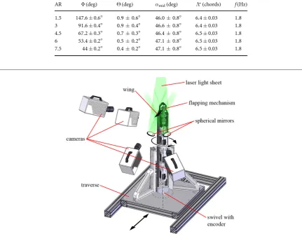
Flowfield measurements were acquired using a high-speed stereo PIV system comprised of a 527 nm 1 kHz Nd:YLF laser(Litron LDY-300PIV, Litron Lasers Ltd, UK) and four 1024 ×1024 px high speed cameras (Photron SA3, Photron Ltd). As illustrated infigure4, the measurement plane (i.e. the light sheet) was positioned such that it was aligned with the wing chord when the wing was at a pre-defined position in the wing stroke, at which point measurements were triggered by the flapperatus. This enabled repeated measurements and ensemble(or phase-locked) aver-aging of the flow fields. The light sheet measured
∼1.5 mm in thickness and was produced using a set of optics comprising a spherical and cylindrical lens. Olive oil seeding particles of~1 mm in diameter were produced with a compressed air aerosol generator. The laser pulse separation was set such that particles would travel no further than 25% of the light sheet thickness in the out-of-plane direction (previously shown to be optimal (Keane and Adrian 1991)), assuming a maximum out-of-plane velocity of two
times the mean wingtip speed that has been reported
elsewhere (Lu and Shen 2008, Phillips and
Knowles2013).
Four cameras were used to measure above and below the wing simultaneously(figure4). To illumi-nate the shadow cast by the wing, a pair of spherical lenses were arranged∼5 wing chords below the stroke plane to reflect the light sheet onto the underside of the wing. The upper and lower pair of cameras werefitted with 105 mm lenses(AF Nikkor, f/2.8), and 180 mm lenses(AF Nikkor, f/3.5)respectively via Scheimpflug mounts(Westerweel1997). The PIV system was syn-chronized with a high-speed controller and operated by DaVis 7.2.2 software(LaVision UK Ltd, Oxford-shire). Spatial calibration of the four camera views was achieved using a dual-plane 105×105 mm calibration grid. Small misalignment between the grid plate and the light sheet was corrected with a disparity map rou-tine(Willert1997, Scaranoet al2005).
The flapperatus was mounted on a swivel and a traverse as shown infigure4. The swivel axis of rota-tion coincided with the wing stroke centre of rotarota-tion, and wasfitted with a digital encoder that recorded the swivel angle to within±0.1°. This enabled measure-ments at different points in the wing stroke to be achieved without reorienting the PIV measurement frame of reference. The traverse allowed the wing to be
translated relative to the measurement plane in 1 mm increments during measurements, resulting in a dense volume of velocity data. The traversing speed was neg-ligible compared to the mean wingtip speed(0.12% of
¯
vtip), nevertheless, following the arrival at a new
span-wise location,five flapping periods were allowed to elapse before measurements were resumed. This wait time was found to be more than sufficient such that any effects on theflowfield from intermittently traver-sing the wing were excluded. The resulting measure-ment volume was comprised of PIV velocity data planes taken every 1 mm from 2 mm inboard of the wing root to 15 mm beyond the wingtip for each wing, with three repeat measures at each spanwise location.
3. Data processing and analysis
3.1. PIV processing
The raw image pairs were pre-processed in DaVis 8.0.8 (LaVision UK Ltd, Oxfordshire)to identify the line of intersection of the laser light sheet with the wing by locating areas above a specified intensity threshold. A mask was applied to this region to exclude it from processing. We calculated a sliding minimum pixel intensity across the image over the three samples taken at each spanwise location and subtracted these
Table 1.Kinematic parameters.
AR Φ(deg) Θ(deg) amid(deg) L(chords) f(Hz)
1.5 147.6±0.6° 0.90.6 46.00.8 6.4±0.03 1.8 3 91.6±0.4° 0.90.4 46.60.8 6.4±0.03 1.8 4.5 67.2±0.3° 0.70.3 46.40.8 6.5±0.03 1.8 6 53.4±0.2° 0.50.2 47.10.8 6.5±0.03 1.8 7.5 44±0.2° 0.40.2 47.10.8 6.5±0.03 1.8
intensities from the individual sample images. This effectively removed reflections from the laser on the wing and background objects, but retained the particle images. Images were subjected to a stereo cross-correlation algorithm with an initial interrogation window size of 64 × 64 px progressing to a final 16×16 px window size. For each of these windows, two passes were made with a 50% overlap and deformable windows. Between passes, the median
filter proposed by Westerweel (1994) was used to identify and remove spurious vectors, where vector components of twice the rms value of their neighbour-ing components were considered spurious. After processing, any regions with empty spaces, aside from the masked region, were filled up via interpolation. Vector maps were then averaged over the three samples per spanwise location, and assembled into a dense 3D volume of velocity data for each of the measured instances through the wing stroke.
3.2. Vortex identification
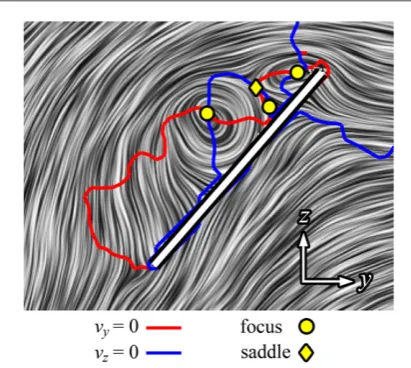
We objectively identified in-plane critical points by locating zero-crossing points for the velocity profiles in the xand y directions (Knowles et al 2006). An example is given in figure 5, where intersections betweenvy=0 andvz=0 contour lines mark critical point locations. In this process, critical points are automatically classified into different types (i.e. focuses, saddles)using criteria outlined by Chonget al (1990). This technique was applied to everyxy,yzand xz plane in the assembled volume of velocity data, resulting in a collection of 3D coordinates of critical points for a given position in the wing stroke. The 3D coordinates of foci were joined into lines representing vortex axes using a custom algorithm exploiting the fact that the 3D vorticity vectors along a vortex axis are tangent to the local path of the axis. With the identified axes, vortex diameter, circulation and axial vorticity were determined at each point along an axis by examining the velocity profile in a plane perpendicular to the local axis direction at a given point. Here the
vortex diameterDis taken as the diameter of the rigid-body rotation region in the local Rankine vortex velocity profile, and its circulation isG =pDvtwhere
vtis the tangential flow velocity at the extent of the
rigid-body rotation region. Details of the employed vortex axis identification method are given elsewhere (appendix,(Phillips2011)).
3.3. line integral convolution(LIC)and skin friction lines
Flow field velocity measurements were achieved to within ~1 mm from the wing surface owing to the method we used forfiltering out reflections from the wing surface(section3.1). Without this step, measure-ments close to the surface are less reliable because the high pixel intensities of the reflections are weighted higher than lower intensities in the correlation func-tion. The reflection removal method effectively reduces them to near-zero pixel intensity leaving only the particles. Measurements near the surface are further complicated by the fact that velocity gradients in the boundary layer lead to bias errors. This has been characterized by Kähleret al(2012)who found that bias errors decrease to zero at a distance of one half of the interrogation window size from the surface and beyond. Thefinal interrogation window size used in the present study corresponds to 1.7 mm. Thus, vectors as close as 0.85 mm from the surface are deemed valid and with negligible bias errors. With this in mind,flow velocity measurements at a conservative distance of 1 mm from the wing surface were used to visualize near-surfaceflows within the boundary layer. The result is a vectorfield, to which LIC can be applied. LIC was originally presented by Cabral and Leedom (1993), and the method employed here is described in detail elsewhere(Lawsonet al2005). Additionally, LIC was applied to chordwise slices through theflowfield.
4. Results and discussion
First, we present the 3Dflow development versus AR, followed by examination of individual chordwise planes to describe further detail of the LEV diameter and strength. Last, the LEV-generated lift force will be presented and discussed along with corresponding lift coefficient values versus AR.
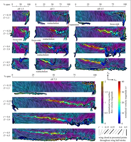
Figure6depicts the formation and evolution of the
flowfield throughout the wing half-stroke for each AR. The view is of the upper surface of the wing plan-form, looking down on the wing along thezwaxis in
vorticity magnitude given by∣w∣. Here vorticitywis normalized by the ratio ofv¯tip c w¯ ( =wc v¯ ¯ )tip .
Complementing figure 6, figure 7 presents the chordwise LEV axis position(figure7(a))and height above the wing surface(figure7(b))for all ARs at the same instants in the half-stroke.
An interpretation of the flow topologies from the near-surface skin friction lines infigure6can be pro-vided by previously established separation patterns. These are derived from local solutions to the Navier– Stokes equations and use critical points such as foci, sad-dles, sinks and sources(Hornung and Perry1984, Perry and Chong1987, Chonget al1990). Such analysis has been applied previously to insectflow topologies by qua-litative smoke-wire visualizations (Srygley and Tho-mas2002, Thomaset al2004, Bomphreyet al2009), and
on flowfield measurements of the LEV growth and detachment process on plunging aerofoils (Rival et al2014). Two of the most common patterns which will be referred to hereon are the open negative bifurca-tion line separabifurca-tion and the Werlé–Legendre separabifurca-tion illustrated infigure8(Hornung and Perry1984). The former consists of aflow convergence to a separatrix (figure8(a)), while in the latter, theflow spirals into a focus plus sink(figure8(b))where it leaves the surface encircling a vortex axis originating from the focus-sink centre(Hornung and Perry1984).
4.1. 3Dflow development
4.1.1. Early in the half-stroke
As seen infigure 6, the generalflow development is qualitatively very similar from AR = 1.5 to 7.5
Figure 6.3Dflow topology evolution throughout half-stroke versus AR; select planform views shown for AR=1.5, 3, 4.5 and 7.5 wing upper surface with near-surface skin friction lines coloured by in-plane velocity magnitude(normalized byv¯tip); major vortex
throughout the stroke. At the start of the half-stroke, a trailing-edge vortex(TEV)forms and sheds and the primary LEVfirst appears outboard around thefirst 1.3 tip chords of travel(t=0.15seefigure7). At this stage, for all ARs the LEV appears to merge with the TiV and an open negative bifurcation separation line is present close to the leading edge with a reattachment line further aft marking the LEV ‘foot-print’. For clarity, approximate secondary separation and reattachment lines(see section3)are marked in
figure6for AR=3only, although the same pattern can be seen throughout the stroke for each AR(with the exception of the end-of-stroke position for AR=1.5). Att=0.15, the remainder of the wing area that is not taken up by the LEV footprint consists of chordwise attachedflow directed toward the trail-ing edge.
4.1.2. Midstroke and after
As the wing proceeds to mid-stroke at t =
l =
( )
0.25 3.25 and beyond tot =0.4(l =5.9)at the onset of pitch reversal, the primary LEV continu-ously grows in size and encroaches further inboard (figure 6). Correspondingly, the reattachment line shifts aft and inboard. Over this period, for higher AR
the outboard portion of the LEV axis is generally further from the leading edge and further above the wing surface(figures7(a)and(b)). This indicates that, outboard, the LEV core position is less stable through-out the stroke as AR increases, possibly resulting in LEV detachment, which will be discussed further in the next section.
The LEV takes an arch-shaped form with its out-board end appearing to be anchored on the wing sur-face. This is consistent with observations made by Carr et al (2013) who reported an arch-shaped LEV for AR=2 and 4 for a rotating wing at afixed45angle of attack. Our results illustrate that this phenomenon extends up to at least AR=7.5. The existence of an arch-shaped axis is reinforced by the near-surface skin friction lines infigure6which suggest the presence of a focus-sink on the wing surface near the wingtip. From this critical point, the outboard end of the LEV axis emanates. An example of the focus-sink is labelled for
= t =
AR 4.5 at 0.25(figure6), and similar indica-tions of this feature are seen elsewhere except for AR=1.5 and 3 att=0.4where their axes appear less arch-like infigure7(b).
From the previous observations it appears that prior to mid-stroke, for all ARs the inboard end of the LEV axis originates from an open negative bifurcation line type separation(from the primary separation line along the leading edge)and the outboard end origi-nates from a Werlé–Legendre type separation com-pleting the arch. Post mid-stroke, this remains the case for AR>3 until the onset of stroke reversal, whereas for AR < 3 the LEV axis outboard becomes con-tinuous with the TiV axis and, thus, has no terminus on the wing surface. Furthermore, for AR=1.5 an additional focus-sink appears near the leading edge late in the half-stroke(labelled infigure6), suggesting that for AR=1.5, the inboard end of the LEV axis transitions to a Werlé–Legendre type separation.
Figure 7.LEV position throughout half-stroke versus AR;(a)chordwise position from leading edgeywand(b)above wing surface
zw shown at select points corresponding tofigure6; coordinates are normalized by the wing chord; black dashed line represents the
trailing edge.
Transitional states of separation over hawkmoth wings had been postulated elsewhere (Bomphrey et al2005)and visualized over bumblebees(Bomphrey et al2009); this is further evidence thatflow topologies can be highly dynamic throughout the wing stroke cycle.
The trailing vortices also have differing origins, the TiV originates from the open negative bifurcation separation line along the wingtip whereas the root vor-tex originates from a focus-sink on the wing surface (e.g.AR=3,t=0.4infigure6)and is, therefore, a Werlé–Legendre type separation. It should be noted that a third type of separation pattern referred to as open U-shaped separation is possible for the LEV in which the LEVs on adjacent wings are continuous and extend over the insect’s body, as suggested by Luttges (1989)and visualized over insects(Srygley and
Tho-mas 2002, Thomas et al 2004, Bomphrey
et al2005,2009, Bomphrey2006).
4.1.3. LEV detachment
Local LEV detachment in the present study is con-sidered to occur when theflow at the trailing edge reverses and initiates the formation of a TEV. In previous detailed CFD studies by Wilkins(2008), LEV detachment on a translating wing at high angle of attack was seen to be immediately preceded by such a reversal generating a TEV. This is further supported in experimental studies by Rivalet al(2014) characteriz-ing LEVflow topology, where it was shown that when the stagnation point aft of the LEV merges with the stagnation point at the trailing edge, the merged (saddle)point lifts off the wing initiating LEV detach-ment. Interrogation of the trailing edge (~0.03c
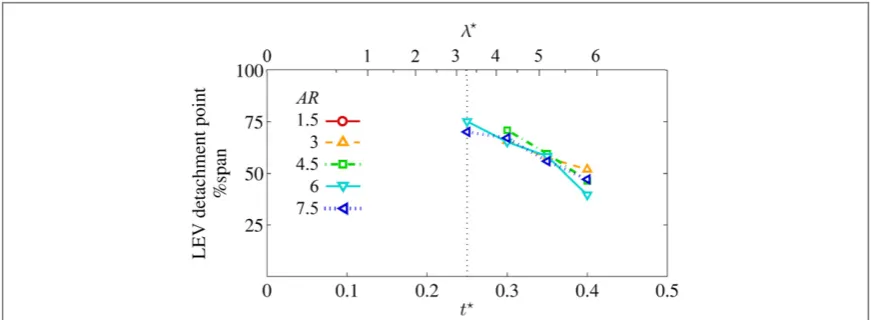
normal distance above trailing edge)throughout the half-stroke for the onset offlow reversal yields the LEV detachment point for each AR as illustrated infigure9. For the higher ARs, 6 and 7.5, LEV detachment initiates at mid-stroke, at t=0.25, whereas for AR=3 and 4.5 it occurs shortly after att=0.3, and no detachment is detected at all for AR = 1.5.
Interestingly, despite the wide range in wing length, initial detachment occurs for AR>1.5 around the same spanwise location of approximately 70% span. This is in close agreement with the numerical simula-tions of Harbiget al(2013)who found that the LEV separates at 70% span over the examined range of AR = 2.91–7.28. In addition, the computational studies of Liuet al(1998)reported LEV detachment outboard of a vortex breakdown point at 75% span on a hawkmoth wing. Returning tofigure9, beyond mid-stroke the LEV detachment point progresses inboard at the same rate for each AR (>1.5)until it reaches approximately mid-span at t =0.4, the onset of pitch reversal. Subsequently, the flow reattachment point shifts towards the leading edge due to the influence of the TEV andflow towards the trailing edge is restored along the span. Lentink and Dickinson claimed that the LEV will be continually stable for a revolving wing forRoof( )1 , whereRowas equated to aspect ratio, implying the condition of AR of( )1
for a stable LEV(Lentink and Dickinson2009). In the present study, all ARs are of this order of magnitude, and our results are consistent with their claims in the sense that the majority of the LEV is stable and remains attached(particularly inboard where the local Rois lower)even up to the end of the stroke. However, the story is more complex, as it is shown here and also elsewhere(Harbiget al2013)that the LEV outboard becomes unstable for AR>1.5 even though the general condition ofAR=( )1 is met.
4.1.4. End of half-stroke
Finally, beyond t=0.4, the wing pitches up and continues to decelerate until it is at rest at the end of half-stroke (t=0.5; l=6.5). As can be seen in
figure6, for AR>1.5a strong TEV is present along the trailing edge at the end of half-stroke, which coincides with pitch reversal. As a consequence of the TEVʼs presence, the reattachment line migrates toward the leading edge(e.g. AR=3 infigure6)such that it lies between the LEV and TEV footprints for
>
AR 1.5.Also at this stage, no clear LEV axis is found beyond approximately 60% span because the LEV beyond this point has detached and is likely to have broken down. Inboard, however, the LEV position relative to the wing has remained virtually unchanged sincet=0.4(figures7(a)and(b)). For AR=1.5 the picture is slightly different at the end of the half-stroke. First, no clear TEV axis is found, probably because the
TEV for AR = 1.5 is much smaller and weaker
compared to the other ARs. Furthermore, the LEV axis is visible in the outboard region and there is no obvious reattachment line. Compared witht=0.4,
the LEV axis for AR= 1.5 has shifted towards the leading edge but is relatively the same distance above the wing(figures7(a)and(b)).
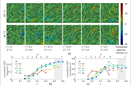
4.2. Chordwise planes and LEV characteristics
We will now addressflow development versus AR by examining chordwise planes through the flowfield along with the LEV diameter and circulation. Figures10–12present these results at 25%, 50% and 75% span respectively. Eachfigure shows chordwise planes of instantaneous LIC streamlines, coloured by normalized spanwise vorticity wx for AR=1.5 and 7.5, along with plots of LEV normalized diameterD
and circulation G throughout the half-stroke. Here
circulation Γ is normalized according to
G = G (¯ ¯ )cvtip. In some cases, these plots continue
into the next half-stroke (shaded region)where the LEV can be tracked as it persists under the wing into the subsequent half-stroke.
The chordwise planes shown in figures 10(a)– 12(a), show again that the generalflow development is qualitatively very similar from AR=1.5 to 7.5. Despite this general similarity there are a number of clear trends that arise as AR increases, which will be out-lined below.
First, as AR increases, the primary LEV across the span is generally larger, with stronger circulation. As seen infigures10(b)and(c)at 25% span it is clearly larger in size in the second half of the half-stroke for higher AR yet normalized circulation values are simi-lar. At 50% span infigures11(b)and(c)the LEV dia-meters are more comparable but circulation is higher in the second portion of the half-stroke which implies greater core vorticity for higher AR at this region on the span. Finally, at 75% span,figures12(b)and(c), the increase in both LEV size and circulation with AR are strikingly clear.
Due to the general increase in LEV size and strength with AR, particularly in the second half of the half-stroke, the inboard portion of the LEV continues to persist under the wing well into the subsequent half-stroke for higher ARs. This can be seen clearly in
figure 10(a) at 25% span for AR= 7.5 in approxi-mately thefirst chord of travel by the wing tip. A simi-lar observation was made by Liuet al(1998)who, in a computational study on a hawkmoth wing, saw the LEV deform into a‘hook-shaped vortex’during supi-nation which remained present until the wing began to translate into the upstroke. Furthermore, Poelmaet al (2006)reported regions of vorticity associated with the
LEV that convect off the trailing edge during pitch reversal. The persistence of the LEV under the wing will negatively impact lift production into the next
half-stroke as it decreases the pressure on the lower wing surface. This negative effect is compounded by the fact that this LEVʼs presence beneath the wing
Figure 11.LEV development at 50% span;(a)select chordwise planes of instantaneous streamlines for AR=1.5 and 7.5; wing chord is denoted by white line;(b)normalized LEV diameterDand(c)normalized LEV circulationGthroughout half-stroke
appears to delay the formation of the new primary LEV, which can be seen by comparing the LEV size and vorticity in the chordwise planes between AR=1.5 and 7.5 fort =0.1 0.15– at 25% and 50% span infigures10(a)and11(a), respectively. The pri-mary LEV forms sooner for the lower AR=1.5. This is likely to be a result of the fact that the LEVʼs presence under the wing for a higher AR induces aflow at the leading edge which modifies the direction of the local
flow in such a way that the effective angle of attack is reduced and separation is consequently suppressed. The effect can be seen by comparing the direction of incidentflow to the leading edge att =0.1between
AR = 1.5 and 7.5 for 25% and 50% span in
figures10(a)and11(a), respectively.
The observed delay in LEV formation is also apparent in the trends of diameter and circulation growth at 25% and 50% span(figures10(b),(c)and 11(b),(c)respectively), where it is seen that for thefirst half of the half-stroke, the inboard portion of the wing for AR=1.5 possesses a larger and stronger primary LEV compared to the other ARs. Even though LEV formation is delayed in this manner, the LEV diameter and circulation for higher ARs‘catch-up’as their rates of change are steeper for thefirst half of the half-stroke and beyond, particularly at the mid-span region.
4.2.1. Secondary and tertiary LEV
In the chordwise planes presented here, additional minor vortex structures are visible that either had no clear 3D vortex axis or were purposely omitted in
figure 6. Notably, from approximately mid-stroke onwards in the outboard region, there are indications of a smaller secondary LEV close to the leading edge that has the same sense of rotation as the primary LEV (figures11(a)and12(a)). Dual LEVs such as these have been reported on butterflies (Srygley and Tho-mas2002)and, as seen from the present results, it is a feature that is present for all ARs. This is consistent with observations by Luet al(2006)who reported dual LEVs with the same sense up to their highest tested aspect ratio of 10, and thus concluded that thisflow
feature is insensitive to AR. Dual LEVs have been observed numerous times, in both experimental (Lentink and Dickinson 2009), and numerical (Liu et al1998, Harbiget al2013)studies. Furthermore, we have sufficient resolution to observe a tertiary LEV located between the primary and secondary LEVs and with an opposite rotational sense. This occurs at all ARs (for example, at t=0.4 for AR = 7.5 in
figure11(a)). The tertiary structure has been reported by Harbiget al(2013)at Reynolds numbers of 750 and above across a range of aspect ratios(2.91–7.28), and elsewhere(Phillips2011). In delta wing aerodynamics this tertiary vortex is typically referred to as a secondary LEV.
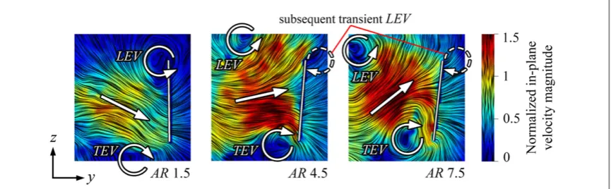
4.2.2. Transient LEV at stroke reversal
At the end of the half-stroke a jet forms between the TEV and the shedding LEV. At lower ARs this jet is directed downwards, while at higher ARs the jet is angled upwards in the outboard region of the wing (figure 13). This shift in jet angle is due to the LEV having convected further away from the wing in the higher AR cases. To compound matters, the TEV is formed earlier in the higher AR cases, which can be seen by comparingt=0.4between AR=1.5 and 7.5 infigure12(a). The TEV is also bigger and stronger towards the end of the half-stroke for higher ARs which, combined with a stronger outboard LEV, creates a greater induced jet between them(figure13).
As the wing reverses, it is momentarily stationary in the global frame of reference but moving relative to its own inducedflow. When the LEV/TEV jet is direc-ted upwards, as it is for our higher AR wings, vorticity can be shed from the leading edge over the new upper surface when the wing speed is zero. This vorticity, which forms on the outboard section of the wing, can be seen infigure12(a), AR=7.5, duringt=0 0.1,– as the wing tip accelerated through itsfirst half chord length of travel. After this shedding event, the primary LEV soon forms. This transient LEV associated with stroke reversal is aflow feature found for AR=3 and above, and occurs in the outboard region where the
primary LEV has already detached. It can be thought of as a form of‘wake capture’. Relatively speaking, the incidentflow is directed towards the leading edge in a fashion akin to that experienced by the trailing edge early in the wing stroke when a TEV is generated. Thus, the transient LEV forms and sheds in much the same way that the TEV does at the start of the wing half-stroke.
4.3. LEV lift
The lift generated by an accelerating wing at high angle of attack is the combination of two parts: circulatory lift contained in bound circulation and external vortices, and non-circulatory lift from added mass effects in the acceleration phase. Of the two parts, circulatory lift is more significant as it generates the majority of the lift force throughout a wing stroke (Maybury and Lehmann2004). In studies by Pitt Ford and Babinsky(2013), it was found that the value for bound circulation that gave the bestfit between their potentialflow model and experimentalflowfield data from a translating wing was small. This led them to the conclusion that the majority of the circulation is contained in external vortices, namely, the LEV. Therefore, the circulatory lift generated by the LEV throughout a wing stroke comprises the majority of the lift produced and, thus, provides a good measure of the total lift.
Here, for a given point in the half-stroke, the circu-latory lift of the LEV along the span can be calculated by the varying circulation values along the vortex axis and the local instantaneous wing speed according to the Kutta–Joukowski theorem. The result is a span-wise loading distribution which is then integrated to obtain the lift force and the lift coefficientCLusingv¯tip
as the characteristic velocity. We calculated the lift coefficient, using the primary LEV only, for each AR throughout the wing stroke(figure14(a)). Including the non-circulatory contribution to lift from added
mass(Maybury and Lehmann 2004)has a negligible effect because it is comparatively small; for all ARs, the time-averaged lift coefficient from added mass was at most 1.1% of the corresponding circulatory lift coeffi -cient from the LEV.
Lift steadily increases until approximately mid-stroke, and then declines. For the higher ARs(greater than 3), lift forces become negative into the next half-stroke(shaded region infigure14(a))as the LEV per-sists on the wing’s underside.
Time-averaged lift coefficients are generally larger for higher AR(figure14(b))but this trend does not continue indefinitely. Mean lift steadily increases with AR up to a value of 6 and then declines slightly. The decline in mean lift coefficient atAR>6is explained
by the drop in LEV circulation after AR = 6
(figures 11(c), and 12(c)). Circulation drops at the highest ARs as the LEV detaches. This phenomenon leads to a higher lift coefficient for AR=6 than for AR = 7.5 in the latter part of the half-stroke (t>0.25; figure 14(a)), and thus, a higher mean
value for the entire stroke. Consistent with our results, Harbiget alʼs computational study(Harbiget al2013) found that for span-based Reynolds numbers
> ~
ReR 1500 (c.f. ReR=2500 here) the mean lift coefficient increases with AR and remains fairly con-stant in some cases up to a value of approximately 5, after which it decreases. The authors attributed this to a decrease in LEV circulation towards the tip beyond
»
AR 5 which resulted from the interaction with trailing-edge vorticity. The present results show peak lift at AR=6, whereas in Harbiget alʼs study lift was seen to decline after AR=5(Harbiget al2013). This difference could arise from the different (fruit fly) wing geometry used, and the different approach of characterizing lift using a computational model versus
calculating LEV circulation from flow field
measurements.
5. Conclusions
The effect of varying wing aspect ratio within, and beyond, the range found in nature was investigated experimentally using high spatial- and temporal-resolution PIV. Qualitatively, theflowfields developed in a similar manner across all wings tested. This was characterized chiefly by the formation of a primary, conical, LEV with an axis that arches above the wing at the outboard end. In most cases, the inboard end of the LEV connected an open negative bifurcation separation line at the leading edge to a Werlé– Legendre focus-sink separation on the wing surface at its outboard end. As the wing half-stroke progressed, the LEV grew in size and strength, with its origin progressing further inboard, forming a larger foot-print on the wing surface accompanied by a shift in the
flow reattachment line inboard and toward the trailing edge. Also common, was the formation of a secondary LEV closer to the leading edge with the same rotational sense as the primary, and a tertiary LEV located in between the two but with an opposite sense of rotation.
As AR increases, the LEV axis outboard shifts fur-ther aft and rises furfur-ther above the wing surface, the result of a larger vortex diameter outboard that ulti-mately leads to earlier detachment in this region. Detachment occurred for AR > 1.5 at mid-stroke (initiating earlier with higher AR) at the 70% span location and moved inboard as the half-stroke pro-gressed. Accompanying advanced LEV detachment with increasing AR was the earlier onset of a TEV, even before pitch reversal, due to the influence of the LEV on theflow at the trailing edge. This led to a stronger LEV/TEV vortex pair that was strengthened and reor-iented at the end of the half-stroke with higher AR. The consequence of this reorientation is a switch in the LEV/TEV-induced jet to a direction towards the lead-ing edge, which then results in a transient LEV form-ing on the outboard region of the wform-ing that sheds quickly as the subsequent wing stroke begins.
As a result of the larger and higher LEV circulation across the span with increasing AR, the inboard por-tion of the LEV(which remains attached)was seen to persist underneath the wing surface into the sub-sequent half-stroke. This had the effect of reducing lift due to the weakenedflow arriving at the leading edge being reoriented in a way that lowered the effective angle of attack and delayed the formation of the pri-mary LEV in the next half-stroke. Thus, the pripri-mary LEV forms sooner for lower ARs; however, for higher ARs the rate of growth of its size and strength are stee-per and it quickly surpasses the lower ARs as the half-stroke proceeds.
The coefficient of circulatory lift generated by the LEV throughout the half-stroke was found to increase monotonically with AR up toAR=6,before declin-ing slightly in the AR =7.5 case. This decline was attributed to a loss in instantaneous lift coefficient in
the second half of the wing half-stroke owing to diminished circulation as the outboard LEV sheds. Thus, increasing aspect ratio initially improves lift through a larger and stronger LEV, however the out-board LEV portion grows too large for the wing chord, becomes unstable, and detaches, leading to reduced overall lift. From these results, it appears that the opti-mal point between these two competing effects is around AR=6 where peak lift is achieved, at least for a rectangular planform. This could explain why insect wing aspect ratios only go as high as∽5(Dudley1999), because increasing AR to this point improves lift per-formance. However, further increases in AR provide no aerodynamic benefit to justify the cost of higher inertial power and the higher muscle torques needed to drive theflapping motion.
Acknowledgments
This work was supported by an EPSRC Career Acceleration Fellowship to R J B (EP/H004025/1). The authors would like to thank Dr Graham Stabler for his invaluable advice and help in the development of the experimental apparatus, and Tony Price and John Hogg for their help with installation of the experimental setup. In addition, the authors would like to thank Dr Toshiyuki Nakata for the use of his insect wing images appearing infigure1(c).
Appendix. Critical point joining algorithm
This appendix describes in more detail the method employed for identifying 3D vortex axes in the measurement volume. Recall from section3.2that the method of Knowleset al (2006) was used to locate critical points from zero-crossing points of in-plane velocity components. In this process, critical points are automatically classified into different types using criteria outlined by Chong et al (1990) for the coefficientsP,Q,Rfrom the characteristic equation of the velocity gradient tensorv(i.e. a focus ifQ>0, or a saddle ifQ<0). In this study, only vortices were of interest, so critical points in the measurement volume not classified as foci were excluded. The remaining points were then joined to form a vortex axis as illustrated by the example in figure A1 using the algorithm outlined subsequently.
The algorithm for joining critical points into a vor-tex axis requires the user manually to select a starting point, from which the axis is constructed in a step-wise manner. The process will be illustrated by way of an example in 2D. FigureA2illustrates an axis comprised of pointsn1and n2, whilen3and n4 are being
con-sidered for the next axis point. Position and vorticity vectors are given by symbols r and w. Referring to
figureA2, for the current pointi(n2)with the previous
point being i−1 (n1), subsequent points j(n n3, 4),
is below 1 mm, andbwi wj, (angle between vorticity
vec-tors at pointi, andj),brj i wj, (angle between position
vector from i to j and vorticity vector at j), and
bri i-1,rj i(angle between position vector fromi−1 to iand position vector fromitoj)are each below the threshold of 75°. Of the points that meet these criteria, the one which has the minimum sum of the distances ∣rj i∣, ∣rj i∣sin(brj i wi, ) and ∣rj i∣sin(brj i wj, ) is
deemed to be the next point on the vortex axis, and the process repeats for the next point. The end of the axis is reached when none of the remaining points meet the initial threshold criteria. These criteria collectively ensure that the deviation of the 3D vorticity vector from the tangent to the local path of the vortex axis is minimized while restricting the vortex axis to turn
through a maximum of 75° between subsequent
points. Although illustrated using a 2D example, this
process was performed in 3D with three-component vectors.
An illustration of the performance of this vortex axis identification method is given in figure A3(a), which presents vorticity vectors along the same
identi-fied vortex axis shown infigureA1, where the vectors faithfully follow the axis trajectory. This is made more clear by comparing the axial component of vorticity and vorticity magnitude(which should be equal)along the axis infigureA3(b), indicating the goodness-of-fit of the identified axis to the true axis. Inspiration was drawn from the method of Singer and Banks(1994) which reconstructs vortex axes in a similar stepwise manner using the direction of the current vorticity vector on an axis to step towards the next axis point set at the pressure minimum in a local cross-sectional plane.
Figure A1.Example result(below)of critical point joining algorithm to form vortex axis(taken from AR=3 at midstroke).
References
Anderson J D 2001Fundamentals of Aerodynamics3rd edn(New York: McGraw-Hill)
Ansari S A, Knowles K andŻbikowski R 2008 Insectlikeflapping wings in the hover: I. Effect of wing kinematicsJ. Aircr.45
1945–54
Bomphrey R J 2006 Insects inflight: direct visualization andflow measurementsBioinsp. Biomim.11–9
Bomphrey R J, Lawson N J, Harding N J, Taylor G K and Thomas A L R 2005 The aerodynamics of Manduca sexta: digital particle image velocimetry analysis of the leading-edge vortexJ. Exp. Biol.2081079–94
Bomphrey R J, Taylor G K and Thomas A L R 2009 Smoke visualization of free-flying bumblebees indicates independent leading-edge vortices on each wing pairExp. Fluids46
811–21
Cabral B and Leedom L C 1993 Imaging vectorfields using line integral convolution‘SIGGRAPH 93’(Anaheim, US)
Carr Z, Chen C and Ringuette M 2013 Finite-span rotating wings: three-dimensional vortex formation and variations with aspect ratioExp. Fluids541–26
Chong M S, Perry A E and Cantwell B J 1990 A general classification of three-dimensionalflowfieldsPhys. Fluids2765–77 Dickinson M H and Götz K G 1993 Unsteady aerodynamic
performance of model wings at low Reynolds numbersJ. Exp. Biol.17445–64
Dickinson M H, Lehmann F O and Sane S P 1999 Wing rotation and the aerodynamic basis of insectflightScience2841954–60 Dudley R 1999The Biomechanics of Insect Flight: Form, Function,
Evolution(Princeton, NJ: Princeton University Press) Ellington C P 1984 The aerodynamics of hovering insectflight: II.
Morphological parametersPhil. Trans. R. Soc.B30517–40 Ellington C P, van den Berg C, Willmott A P and Thomas A L R 1996
Leading-edge vortices in insectflightNature384626–30 Garmann D J and Visbal M R 2012 Three-dimensionalflow
structure and aerodynamic loading on a low aspect ratio, revolving wing42nd AIAA Fluid Dynamics Conf. Exhibit
(AIAA New Orleans, Louisiana, USA)
Granlund K, Ol M, Bernal L and Kast S 2010 Experiments on free-to-pivot hover motions offlat platesFluid Dynamics and Co-located Conf.(Reston, VA: American Institute of Aeronautics and Astronautics)
Harbig R R, Sheridan J and Thompson M C 2013 Reynolds number and aspect ratio effects on the leading-edge vortex for rotating insect wing planformsJ. Fluid Mech.717166–92
Henningsson P and Bomphrey R J 2013 Span efficiency in hawkmothsJ. R. Soc. Interface101–9
Hornung H and Perry A E 1984 Some aspects of three-dimensional separation: I. Streamsurface bifurcationsZ. Flugwiss. Weltraumforsch.877–87
Kähler C, Scharnowski S and Cierpka C 2012 On the uncertainty of digital PIV and PTV near wallsExp. Fluids521641–56 Keane R D and Adrian R J 1991 Optimization of particle image
velocimeters: II. Multiple pulsed systemsMeas. Sci. Technol.2
963–74
Knowles R D, Finnis M V, Saddington A J and Knowles K 2006 Planar visualization of vorticalflowsProc. Inst. Mech. Eng.G
220619–27
Lawson N J, Finnis M V, Tatum J A and Harrison G M 2005 Combined stereoscopic particle image velocimetry and line integral convolution methods: applications to a sphere sedimenting near a wall in a non-NewtonianfluidJ. Vis.8
261–8
Leibovich S 1984 Vortex stability and breakdown: survey and extensionAIAA J.221192–206
Lentink D and Dickinson M H 2009 Rotational accelerations stabilize leading edge vortices on revolvingfly wingsJ. Exp. Biol.2122705–19
Liu H, Ellington C P, Kawachi K, van den Berg C and Willmott A P 1998 A computationalfluid dynamic study of hawkmoth hoveringJ. Exp. Biol.201461–77
Lu Y and Shen G X 2008 Three-dimensionalflow structures and evolution of the leading-edge vortices on aflapping wing
J. Exp. Biol.2111221–30
Lu Y, Shen G X and Lai G J 2006 Dual leading-edge vortices on
flapping wingsJ. Exp. Biol.2095005–16
Luo G and Sun M 2005 The effects of corrugation and wing planform on the aerodynamic force production of sweeping model insect wingsActa Mech. Sin.21531–41
Luttges M 1989 Accomplished insectfliersFrontiers in Experimental Fluid Mechanics(Lecture Notes in Engineeringvol 46)ed M Gad-el Hak(Berlin: Springer)pp 429–56
Maxworthy T 1979 Experiments on the weis-fogh mechanism of lift generation by insects in hoveringflight: I. Dynamics of the ‘fling’J. Fluid Mech.9347–63
Maybury W J and Lehmann F O 2004 Thefluid dynamics offlight control by kinematic phase lag variation between two robotic insect wingsJ. Exp. Biol.2074707–26
Muijres F T, Johansson L C, Barfield R, Wolf M, Spedding G R and Hedenström A 2008 Leading-edge vortex improves lift in slow-flying batsScience3191250–3
Perry A E and Chong M S 1987 A description of eddying motions andflow patterns using critical-point conceptsAnn. Rev. Fluid Mech.19125–55
Phillips N 2011 Experimental unsteady aerodynamics relevant to insect-inspiredflapping-wing micro air vehiclesPhD Thesis
Cranfield University
Phillips N 2013 Three degree-of-freedom parallel spherical mechanism for payload orienting applicationsUK Patent
2464147
Phillips N and Knowles K 2013 Formation of vortices and spanwise
flow on an insect-likeflapping wing throughout aflapping half cycleAeronaut. J.117471–90
Pitt Ford C W and Babinsky H 2013 Lift and the leading-edge vortex
J. Fluid Mech.720280–313
Poelma C, Dickson W B and Dickinson M H 2006 Time-resolved reconstruction of the full velocityfield around a dynamically-scaledflapping wingExp. Fluids41213–25
Rival D, Kriegseis J, Schaub P, Widmann A and Tropea C 2014 Characteristic length scales for vortex detachment on plunging profiles with varying leading-edge geometryExp. Fluids551–8 Scarano F, David L, Bsibsi M and Calluaud D 2005 S-PIV
comparative assessment: image dewarping+misalignment correction and pinhole+geometric back projectionExp. Fluids39257–66
Singer B and Banks D 1994 A predictor-corrector scheme for vortex identificationTechnical ReportNASA Contractor Report 194882, ICASE Report No. 94-11 NASA Langley
Srygley R B and Thomas A L R 2002 Unconventional lift-generating mechanisms in free-flying butterfliesNature420660–4 Thomas A L R, Taylor G K, Srygley R B, Nudds R L and
Bomphrey R J 2004 Dragonflyflight: free-flight and tethered
flow visualizations reveal a diverse array of unsteady lift-generating mechanisms, controlled primarily via angle of attackJ. Exp. Biol.2074299–323
Usherwood J R and Ellington C P 2002a The aerodynamics of revolving wings: I. Model hawkmoth wingsJ. Exp. Biol.2051547–64 Usherwood J R and Ellington C P 2002b The aerodynamics of
revolving wings: II. Propeller force coefficients from mayfly to quailJ. Exp. Biol.2051565–76
van den Berg C and Ellington C P 1997 The three-dimensional leading-edge vortex of a‘hovering’model hawkmothPhil. Trans. R. Soc.B352329–40
Videler J J, Stamhuis E J and Povel G D E 2004 Leading-edge vortex lifts swiftsScience3061960–2
Warrick D R, Tobalske B W and Powers D R 2005 Aerodynamics of the hovering hummingbirdNature4351094–7
Weis-Fogh T 1964 Biology and physics of locustflight: VIII. Lift and metabolic rate offlying locustsJ. Exp. Biol.41257–71 Weis-Fogh T 1973 Quick estimates offlightfitness in hovering
animals, including novel mechanisms for lift production
J. Exp. Biol.59169–230
Westerweel J 1994 Efficient detection of spurious vectors in particle image velocimetry dataExp. Fluids16236–47
Westerweel J 1997 Fundamentals of digital particle image velocimetryMeas. Sci. Technol.81379–92
Wilkins P C 2008 Some unsteady aerodynamics relevant to insect-inspiredflapping-wing micro air vehiclesPhD Thesis
Cranfield University
Wilkins P C and Knowles K 2009 The leading-edge vortex and aerodynamics of insect-basedflapping-wing micro air vehiclesAeronaut. J.113253–62
Willert C E 1997 Stereoscopic digital particle image velocimetry for application in wind tunnelflowsMeas. Sci. Technol.81465–79 Willmott A P and Ellington C P 1997 The mechanics offlight in the
hawkmoth manduca sexta: I. Kinematics of hovering and forwardflightJ. Exp. Biol.2002705–22
Wojcik C and Buchholz J 2012 The dynamics of spanwise vorticity on a rotatingflat bladeAerospace Sciences Meetings(Reston, VA: American Institute of Aeronautics and Astronautics) Woods M I, Henderson J F and Lock G D 2001 Energy requirements
for theflight of micro air vehiclesAeronaut. J.105135–49 Żbikowski R 1999 Flapping wing autonomous micro air vehicles: