Robust Haebara Linking for Many Groups in the Case of Partial Invariance

Robust Haebara Linking for Many Groups in the

Case of Partial Invariance

Alexander Robitzsch1,2*

1 _{IPN – Leibniz Institute for Science and Mathematics Education, Kiel, Germany} 2 _{Centre for International Student Assessment (ZIB), Kiel, Germany}

* Correspondence: [email protected]

Abstract:The comparison of group means in item response models constitutes an important issue in empirical research. The present article discusses an extension of Haebara linking by proposing a flexible class of robust linking functions for comparisons of many groups. These robust linking functions are particularly suited to item response data that are generated under partial invariance. In a simulation study, it is shown that the newly proposed robust Haebara linking approach outperforms existing approaches of Haebara linking. In an empirical application using PISA data, it is illustrated that country means can be sensitive to the choice of linking functions.

Keywords:linking, item response model, 2PL model, Haebara linking, differential item functioning, partial invariance

1. Introduction

One major goal of empirical studies in psychology and education is to compare cognitive outcomes across many groups. For example, the programme for international student assessment (PISA; [1]) provides international comparisons of student performance for a large group of countries (72 countries in PISA 2015). A major obstacle to these comparisons is that cognitive tests often show differential item functioning (DIF; [2]).

In this article, we propose a robust variant of Haebara linking [3] for many groups. We use a two-parameter logistic model (2PL) item response model to introduce the methodology. It is shown that approximately unbiased group comparisons can be conducted with robust Haebara linking when group-specific subsets of items show DIF (i.e., partial invariance). Importantly, no additional steps for identifying items with DIF are needed; items that possess DIF are essentially treated as outliers [4,5] in the linking procedure.

The paper is structured as follows. Section2describes the 2PL model under partial invariance. Section3introduces the robust Haebara linking method. In Section4, the proposed method is evaluated in a simulation study. Section5presents an empirical example of PISA data. Finally, Section6concludes with a discussion that focuses on limitations and potential gaps for future research.

2. 2PL Model with Partial Invariance

In the following, we introduce the concept of partial invariance for multiple groups. ForG groups(g = 1, . . . ,G),Iitems(i= 1, . . . ,I)are administered. It is assumed that a unidimensional item response model holds in each group with group-specific item response functions (IRF)Pig(θ), indicating the probability of a correct item responseXig, conditional on abilityθ. The IRFs in the 2PL model [6] are given as

P(Xig =1|θg) =Ψ(aig(θg−big)), θg∼N(µg,σ_g2) , (1) wherebigare group-specific item difficulties for itemi(i = 1, . . . ,I)in groupg(g =1, . . . ,G), and aigare group-specific item loadings. In this article, we assume uniform DIF [2] that presupposes that

item loadings are invariant across groups, i.e.,ai1=. . .=aiG ≡ai. Group-specific item difficulties are decomposed intobig =bi+eig, wherebiindicates common item difficulties andeigare denoted as uniform DIF effects. In Equation1,Ψdenotes the logistic distribution function, and it is assumed that the abilities within each groupgare normally distributed with meanµgand standard deviationσg.

It is well known that not all DIF effectseigand group meansµgcan be simultaneously identified in the 2PL model (see [7,8]). To resolve the identification issue, the set of items for each group is partitioned into two distinct sets (see [9]). More specifically, we assume that for each groupg, a subset of so-called anchor itemsJA,g ⊂ J = {1, . . . ,I}exists such thateig = 0 for alli ∈ JA,g. The set of biased items is defined asJB,g =J \ JA,g. Biased items are allowed to possess DIF effectseig = 0, which differs from zero. This situation is also referred in the literature as partial invariance [10,11]. If there are no biased items, all item parameters are invariant, which is denoted as full invariance. One central argument in the DIF literature is that items with DIF effects have the potential to bias the estimated ability distributions (i.e., group means or group standard deviations) and should, therefore, not be included in group comparisons (e.g., [1], for arguments in the PISA study, or [12]). Biased estimates of group means can be particularly expected in the case that all DIF effects of items within a group have the same sign (i.e., unbalanced DIF).

In practice, it is not known which items serve as anchor items for groupg. The choice can be based on a substantive basis (e.g., considerations outside of psychometrics, see [13]) or using psychometric methods. In this article, the identification of group means and group standard deviations is conducted using psychometric methods, namely linking methods (see [14–18] for overviews). Linking methods rely on separate scalings for all groups. In more detail, the 2PL model is fitted for each group (under the assumptionθ∼N(0, 1)), resulting in estimated item loadings ˆagand estimated item intercepts ˆbg for all groups. In the second step, estimated parameters(aˆg, ˆbg)are used to determine the vector of group meansµ= (µ1, . . . ,µG)andσ = (σ1, . . . ,σG)standard deviations.

3. Haebara Linking

In this section, we introduce the robust Haebara linking method that determines group means

µ, group standard deviationsσ, common item slopesa= (a1, . . . ,aI), and common item difficulties

b= (b1, . . . ,bI)based on estimated item loadings ˆagand estimated item intercepts ˆbgfor all groups g. A linking functionHis employed that minimizes the distances between group-specific IRFs and aligned common IRFs for computing unknown parameters(µ,σ,a,b)

H(µ,σ,a,b) =

I

∑

G

∑

Z ρ

Ψ(aigˆ [θ−bigˆ ])−Ψ(ai[σgθ−bi+µg])

ω(θ)dθ , (2)

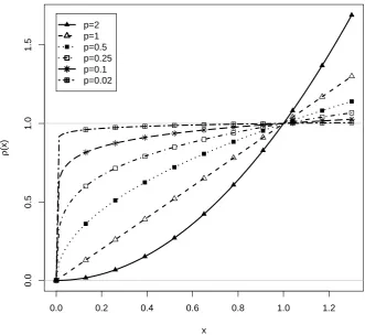
whereρis a loss function, andωis a weighting function that fulfillsR ω(θ)dθ=1. In all subsequent analyses, we choose the standard normal density function as the weighting functionω. Linking based on the functionHin Equation2is referred to as robust Haebara linking and generalizes the originally proposed Haebara linking method for two groups [3] that uses the loss functionρ(x) =x2. He and colleagues [19,20] considered the loss functionρ(x) =|x|for two groups. Haebara linking for multiple groups was investigated in several articles [9,21–23]. In particular, it was shown in [9] that the loss functionρ(x) =|x|was efficient in handling the situation of partial invariance for multiple groups.

0.0 0.2 0.4 0.6 0.8 1.0 1.2

0.0

0.5

1.0

1.5

x

ρ

(x

)

p=2 p=1 p=0.5 p=0.25 p=0.1 p=0.02

Figure 1.Loss functionρ(x) =|x|p_{used in robust Haebara linking with different values ofp.}

In the minimization ofHdefined in Equation2, the unknown parameters can be obtained by setting the first derivatives to 0, i.e., ∂H

∂µ = 0,

∂H ∂σ = 0,

∂H

∂a = 0, and ∂H

∂b = 0. However, the loss functionρ(x) = |x|pis not differentiable for p ≤ 1, and the first derivative must be replaced by a subdifferential. Moreover, due to nondifferentiability ofρ, standard optimization algorithms that rely on derivatives cannot be used. However, in robust Haebara linking, the functionρ(x) =|x|pis replaced by a differentiable approximating functionρD(x) = (x2+ε)p/2using a smallε > 0 (e.g., ε=.001). BecauseρDis differentiable, quasi-Newton minimization approaches can be used that are implemented in standard optimizers in R [24]. The implementation of robust Haebara linking in the sirt [25] package specifies a sequence of decreasing values ofεin the optimization, each using the previous solution as initial values (see [26] for a similar approach).

It should be noted that there are competitive linking methods to Haebara linking. The Stocking-Lord method [27] minimizes the difference of the integrated squared difference of the sum of group-specific IRFs and the sum of aligned common IRFs. There are also alternative linking approaches that directly rely on estimated item parameters instead of IRFs, such as mean-mean linking [16], Haberman linking based on regression modeling [28], invariance alignment [29], and distance-based measures (likeχ2; [30,31]), to name a few. For Haberman linking and invariance alignment, robust alternatives were recently studied [9,32,33]. The linking approach is a two-step method as separate scalings are applied group-wise in the first step. However, it can be shown that one can reformulate the two-step estimation problem as a one-step estimation problem with side conditions [34].

3.1. Estimated Group Means as a Function of DIF Effects

Now, assume that the vector of joint item parametersaandband group standard deviationsσ

ˆ

µg=arg min µ

( _I

∑

ρ

Ψ(aigˆ [θ−bigˆ ])−Ψ(ai[σgθ−bi+µ])

ω(θ)dθ )

. (3)

By using two Taylor approximations, we can formulate the estimated group mean ˆµgas a function of the true meanµgand weighted DIF effectseig. Forp6=1, we get (see AppendixA; EquationA11)

ˆ

µg=µg− 1 p−1

I

∑

wigeig I

∑

wig

, (4)

wherewig =|eig|p−2

R

Wi(θ)ω(θ)dθ, andWiis the information function of itemi. The item-specific weightswigconsist of two factors. First, the factor|eig|p−2_{governs the influence of DIF effects. Items} with large DIF effects eig are down-weighted for p < 2. Second, the factor R

Wi(θ)ω(θ)dθ is the integrated information function with respect toω. The influence of this factor is largest for items with large item loadingsaiand item difficultiesbithat are located in the center of the ability distribution.

We now consider two important special cases of Equation4. Forp=2, we obtain the Haebara linking proposed in [3], and it holds that

ˆ

µg=µg− I

∑

Z

Wi(θ)ω(θ)dθ

eig I

∑

Wi(θ)ω(θ)dθ

. (5)

All DIF effects are weighted according to their item information function. There is no down-weighting of large DIF effects. Forp =0, the estimated group means ˆµgare heavily influenced by items with small DIF effects because items large DIF effectseig are strongly down-weighted. To illustrate the behavior in the situation of partial invariance, let us assume that for the DIF effects of anchor items i ∈ J_A,git holds that|eig| ≈ εwith a small ε > 0 and the DIF effects of biased itemsi ∈ JB,gare much larger than zero in absolute value, i.e.,|eig|>e0. The weights in Equation4are computed as wig =|eig|−2R

Wi(θ)ω(θ)dθ. Further, assume for simplicity thatW≈RWi(θ)ω(θ)dθ, meaning that the integrated information is nearly constant across items. For biased items, we getwig <e₀−2W, and for anchor items it holds thatwig =ε−2W. Inserting these relations in Equation4, we obtain for the bias in estimated group means

Bias(µgˆ ) =−

∑

ε−2eig+

∑

wigeig

∑

i∈J_A,g

ε−2+

∑

wig =−

∑

eig+

∑

ε2wigeig |JA,g|+

∑

i∈J_B,g

ε2wig . (6)

By lettingε→0 in Equation6, we obtain

Bias(µgˆ ) =−

∑

eig |JA,g|

, (7)

and the bias is determined by the DIF effects of the anchor items. As the DIF effects of anchor items were assumed to be small in the derivation, we get unbiased estimated group means in the situation of partial invariance.

4. Simulation Study

4.1. Simulation Design

In this study, we generated dichotomous item responses and investigated the performance of robust Haebara linking for the 2PL model. We adopted a simulation design that was used in [9]. We simulated item responses from a 2PL model forG=9 groups. For each groupg, abilities were normally distributed with meanµgand standard deviationσg. Across all conditions and replications of the simulation, the group means and standard deviations were held fixed (see AppendixBfor values used in the simulation). The total population comprising all groups had a mean of 0 and a standard deviation of 1.

Item responsesXigfor itemiin groupgwere simulated according to the 2PL model

P(Xig =1|θg) =Ψ(ai(θg−bi−Zigδ)) , (8) where DIF effects in item difficulties were defined aseig=Zigδ. The DIF indicator variablesZig had values of 0, 1, or−1, where values different from zero indicated uniform DIF effects. For each country, either all nonzeroZigvalues were 1 or were−1, meaning that all DIF effects had the same direction (i.e., unbalanced DIF). Item loadingsaiwere assumed to be invariant across groups. The DIF effect size was chosen asδ=0.6. A fixed proportionπBof biased items was selected and was equal across groups, i.e.,∑I

i=1|Zig|=IπBfor all groupsg=1, . . . ,G. For example, if 30% out ofI=20 items have DIF effects, 6 items have values ofZigthat differ from zero. The item parameters were held constant across conditions and replications (see AppendixBfor data-generating parameters). In total,I =20 items were used in the simulation.

For each condition of the simulation design,R=300 replications were generated. We manipulated the number of persons per group (N=250, 500, 1000, and 5000). We also varied the proportionπBof biased items with DIF effects (0%, 10%, and 30%).

4.2. Analysis Methods

The performance of robust Haebara linking with powersp = 2, 1, 0.5, 0.25, 0.1, and 0.02 for estimated group means were compared with the scaling approach that relies on full invariance of all item parameters. The approach with full invariance (FI) was specified as a 2PL multiple group item response model.

To identify group means and group standard deviations in the linking procedure, for the first group, the mean was set to 0, and the standard deviation was set to 1. After estimating all group means and group standard deviations, these parameters were transformed to obtain a mean of 0 and a standard deviation 1 for the total sample comprising all groups. These conditions were also fulfilled in the data generating model (see Subsection4.1).

The statistical performance of the vector of estimated means ˆµis assessed by summarizing the

biases and variances of estimators across groups. Letµ = (µ1, . . . ,µG)be a parameter of interest and ˆµ= (µˆ1, . . . , ˆµG)its estimator (i.e., for means and standard deviations). ForRreplications, the obtained estimates are ˆµr = (µˆ1r, . . . , ˆµGr)(r=1, . . . ,R). The average absolute bias (ABIAS) is defined as

ABI AS(µˆ) = 1 G

G

∑

1 R

R

∑

= 1 G

G

∑

Bias(µgˆ ) . (9)

ARMSE(µˆ) = 1 G

G

∑

v u u t1

R R

∑

ˆ

µgr−µg2= 1 G

G

∑

RMSE(µgˆ ) . (10)

In all analyses, the statistical software R [24] was used. Robust Haebara linking was carried out with thesirt::linking.haebara()function in the R package sirt [25]. TheTAM::tam.mml.2pl()function in the R package TAM [35] was used for estimating the 2PL model with marginal maximum likelihood as the estimation method.

4.3. Results

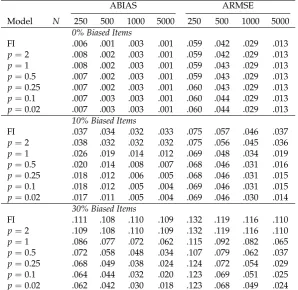
In Table1, average absolute bias (ABIAS) and average RMSE (ARMSE) as a function of sample size are shown. If there are no biased items, all linking methods provided unbiased estimates. As indicated by the ARMSE, there were some efficiency losses by using robust Haebara approaches (p≤1) compared to nonrobust approaches (p =2 or the FI model). The pattern of results for ABIAS and ARMSE for 10% biased items mimic findings for 30% biased items but were less strongly pronounced. Hence, we only describe the results for 30% biased items. The most biased estimates were obtained for the FI model andp=2. Using small values ofpresulted in a reduction of bias. Notably, the smallest biases were obtained forp=0.02. However, biases for robust Haeabara linking were larger for smaller sample sizes. For group sizesN=500, 1000, and 5000, the pattern of RMSE followed that of the bias. Very small values ofpare preferred in terms of most precise estimates. However, forN=250, the smallest ARMSE was obtained forp=0.5. Probably, uncertainty in estimated item parameters adds additional variation and outweighs the smaller bias for smallp.

Table 1. Average Absolute Bias (ABIAS) and Average Root Mean Square Error (ARMSE) of Group Means as a Function of Sample Size

ABIAS ARMSE

Model N 250 500 1000 5000 250 500 1000 5000

0% Biased Items

FI .006 .001 .003 .001 .059 .042 .029 .013

p=2 .008 .002 .003 .001 .059 .042 .029 .013

p=1 .008 .002 .003 .001 .059 .043 .029 .013

p=0.5 .007 .002 .003 .001 .059 .043 .029 .013

p=0.25 .007 .002 .003 .001 .060 .043 .029 .013

p=0.1 .007 .003 .003 .001 .060 .044 .029 .013

p=0.02 .007 .003 .003 .001 .060 .044 .029 .013

10% Biased Items

FI .037 .034 .032 .033 .075 .057 .046 .037

p=2 .038 .032 .032 .032 .075 .056 .045 .036

p=1 .026 .019 .014 .012 .069 .048 .034 .019

p=0.5 .020 .014 .008 .007 .068 .046 .031 .016

p=0.25 .018 .012 .006 .005 .068 .046 .031 .015

p=0.1 .018 .012 .005 .004 .069 .046 .031 .015

p=0.02 .017 .011 .005 .004 .069 .046 .030 .014

30% Biased Items

FI .111 .108 .110 .109 .132 .119 .116 .110

p=2 .109 .108 .110 .109 .132 .119 .116 .110

p=1 .086 .077 .072 .062 .115 .092 .082 .065

p=0.5 .072 .058 .048 .034 .107 .079 .062 .037

p=0.25 .068 .049 .038 .024 .124 .072 .054 .029

p=0.1 .064 .044 .032 .020 .123 .069 .051 .025

p=0.02 .062 .042 .030 .018 .123 .068 .049 .024

Note. N= sample size; FI = linking based on full invariance; p= power used in robust Haebara

To sum up, robust Haebara linking effectively handles situations of partial invariance. Interestingly, values of the power p smaller than 1 are preferred in terms of ABIAS and ARMSE and are superior to previously proposed approaches that usep=2 [3] andp=1 [20].

5. Empirical Example: PISA 2006 Reading Competence

In order to illustrate the choice of different values for the powerpin robust Haebara linking in the case of many groups, we analyzed the data from the PISA 2006 assessment [36]. In this case, groups constitute countries. In this reanalysis, we included 26 OECD countries that participated in 2006 and focused on the reading domain (see [37] for a similar analysis; but see also [9,38,39] for findings using the same dataset). Reading items were only administered to a subset of the participating students, and we included only those students who received a test booklet with at least one reading item. This resulted in a total sample size of 110,236 students (ranging from 2,010 to 12,142 between countries). In total, 28 reading items nested within eight testlets were used in PISA 2006. Six of the 28 items were polytomous and were dichotomously recoded, with only the highest category being recoded as correct. We used seven different analysis models to obtain estimates of the country means: a full invariance approach (concurrent scaling with multiple groups; FI), and robust Haebara linking using powers p=2, 1, 0.5, 0.25, 0.1, and 0.02. For all analyses, the 2PL model was estimated using student weights. Within a country, student weights were normalized to a sum of 5,000, so that all countries contributed equally to the analyses. Finally, all estimated country means were linearly transformed such that the distribution containing all (weighted) students in all 26 countries had a mean of 500 (points) and a standard deviation of 100. Note that this transformation is not equivalent to the one used in officially published PISA publications.

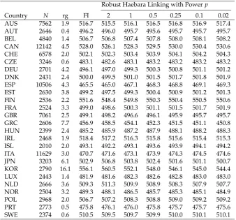
Table 2.Country Means for the Reading Domain for PISA 2006 for 26 Selected OECD Countries Robust Haebara Linking with Powerp

Country N rg FI 2 1 0.5 0.25 0.1 0.02

AUS 7562 1.9 516.7 515.5 516.1 516.5 516.8 516.9 517.4 AUT 2646 0.4 496.2 496.0 495.7 495.6 495.7 495.7 495.7 BEL 4840 1.4 506.7 506.8 507.4 507.8 508.0 508.1 508.2 CAN 12142 4.5 528.0 526.1 528.3 529.5 530.0 530.4 530.6 CHE 6578 2.0 502.1 502.3 503.4 503.9 504.1 504.2 504.3 CZE 3246 0.6 483.1 482.6 483.1 483.2 483.2 483.2 483.2 DEU 2701 4.2 496.1 497.0 499.3 500.3 500.8 501.1 501.2 DNK 2431 2.4 500.0 499.5 501.0 501.5 501.7 501.8 501.9 ESP 10506 4.3 465.5 465.0 467.1 468.3 468.8 469.1 469.3 EST 2630 3.8 499.2 497.5 499.3 500.4 500.9 501.2 501.3 FIN 2536 2.2 551.6 548.4 549.8 550.3 550.4 550.5 550.6 FRA 2524 3.3 499.0 498.6 500.3 501.1 501.5 501.7 501.9 GBR 7061 2.5 499.1 498.2 496.6 496.1 495.9 495.7 495.7 GRC 2606 7.7 456.9 458.5 454.1 452.3 451.5 451.1 450.8 HUN 2399 2.4 485.2 485.9 487.2 487.9 488.1 488.2 488.3 IRL 2468 1.9 518.4 517.2 516.3 515.8 515.6 515.4 515.3 ISL 2010 2.0 493.1 492.2 493.1 493.6 493.9 494.1 494.2 ITA 11629 3.0 470.7 471.6 473.1 473.9 474.3 474.5 474.6 JPN 3203 6.1 502.9 506.8 503.8 502.4 501.6 501.1 500.7 KOR 2790 16.1 556.1 560.5 552.1 548.0 546.1 545.0 544.4 LUX 2443 1.4 481.9 481.6 482.3 482.6 482.8 483.0 483.0 NLD 2666 3.6 509.3 511.3 509.9 508.9 508.3 507.9 507.7 NOR 2504 3.2 489.3 488.1 486.5 485.7 485.3 485.1 484.9 POL 2968 2.0 506.7 507.2 508.3 508.8 509.0 509.2 509.2 PRT 2773 0.5 475.8 476.1 476.0 475.8 475.7 475.7 475.6 SWE 2374 0.6 510.5 509.5 509.7 509.9 510.0 510.1 510.1

In Table2, the country mean estimates obtained from the seven different analysis models are shown. Within a country, the range of country means differed between 0.4 (AUT, Austria) and 16.1 (KOR, South Korea) points (M = 3.2, SD = 3.1) across the different models. These differences between the methods can be traced back to different amounts of country DIF. The model based on full invariance and Haebara linking withp=2 appeared to be similar, resulting in a large correlation of estimated country means (r=.997) and small absolute differences (M=1.2,SD=1.1). In contrast, Haebara linking for p = 2 and p = 0.02 differed quite a lot, resulting in a correlation ofr = .980 and non-negligible absolute differences between methods (M=3.2,SD=3.1). Given that standard errors due to sampling of students in country means in PISA are typically about 3 points, in some cases, differences between different model estimates would provide different statements regarding statistical significance. Interestingly, the country mean estimate for South Korea (KOR) dropped from 560.5 (p=2) to 544.4 (p=0.02). The reason is that robust Haebara linking down-weights items with large DIF effects from the computation of country means. For South Korea, there are four items with large negative DIF effects (a relative advantage) and no items with large positive DIF effects (a relative disadvantage) that are most strongly down-weighted (see [9]). Hence, it can be concluded the choice of a particular linking method has the potential to impact the ranking of countries in PISA (see also [40,41]).

6. Discussion

In this article, we investigated the performance of an extension of Haebara linking in many groups. By using a robust loss function familyρ(x) = |x|p(p >0) it was shown that the method efficiently handles the case of partial invariance.

Originally, Haebara linking has been proposed forp=2 [3] and has been robustified usingp=1 in [20]. Our simulation study showed that power valuespsmaller than 1 has superior performance to the previous proposals in the literature. In more detail, in the case of many groups,pvalues of at most 0.25 are particularly advantageous.

As it is true for all simulation studies, our study has some limitations. First, we restricted the number of groups to 9. For international large-scale assessments like PISA (e.g., [1,36]), the number of groups–countries in this case–are much larger, say 30, or even 50. On the other hand, we believe that the robust Haebara linking method could also be attractive in the case of two groups [42] or a few groups [43]. Second, we only used 20 dichotomous items in the simulation studies. The performance of robust Haebara linking with a very low or higher number of items could be a relevant topic of future research. Third, we restricted ourselves to dichotomous data. Robust Haebara linking could be extended to polytomous items (see, e.g., [44]).

In the simulation study, it was shown that robust Haebara linking shows desirable performance in the situation of partial invariance. However, DIF effects could also be rather unsystematically distributed that cancel on average. This situation is sometimes referred to as approximate invariance (or random DIF, see [32,45–49]). It can be concluded that in the presence of approximate invariance, power values ofp=2 are probably optimal [32,33], and the use of robust Haebara linking can lead to inferior statistical performance.

It should be emphasized that we did not investigate the computation of standard errors in our linking approach. There is ample literature that derives standard error formulas for linking due to sampling of persons (e.g., [44,50–55]) Alternatively, variability in estimated group means due to the selection of items has been studied as linking errors in the literature [38,56–59]. In future research, it would be interesting to accompany robust Haebara linking with error components that reflects these sources of uncertainty. Both analytical standard errors (e.g., [52]) and resampling procedures (e.g., [60]) could be useful in this respect.

measurement waves [61]. One can simply use estimated item parameters resulting from separate scalings of each wave as the input for a linking procedure (see, e.g., [62–69]).

Funding:This research received no external funding.

Conflicts of Interest:The authors declare no conflict of interest.

Abbreviations

The following abbreviations are used in this manuscript:

2PL two-parameter logistic model ABIAS average absolute bias

ARMSE average root mean square error DIF differential item functioning FI full invariance

IRF item response function

PISA programme for international student assessment RMSE root mean square error

Appendix A. Estimated Group Means in Robust Heabara Linking

Appendix A.1. Taylor Approximation of Power Loss Functionρ

Letρ(x) = |x+a|p for p > 0, p 6= 1, and a 6= 0. We now apply a Taylor approximation up to the second order around x = 0. We get ρ0(x) = p|x+a|p−1sign(a) = p|x+a|p−2aand ρ00(x) =p(p−1)|x+a|p−2. Then, we obtain the following approximation

ρ(x) =|x+a|p≈ |a|p+p|a|p−2ax+1

2p(p−1)|a|

p−2_x2 _{. (A1)}

Appendix A.2. Minimization of a Quadratic Function

For the derivation of an estimated group mean in robust Haebara linking, we consider the following quadratic minimization problem

ˆ

µg=arg min µ

A+B(µg−µ) + 1

2C(µg−µ)

2 _{, (A2)}

whereA,B, andCare real numbers. By taking the first derivative in EquationA2, we obtain −B−C(µg−µgˆ ) =0 ⇒ µgˆ =µg+B

C . (A3)

Appendix A.3. Taylor Approximation of Item Response Function with DIF Effects

We now apply a Taylor expansion for the difference of item response functions that appear in robust Haebara linking:

Tig(θ) =Ψ(ai[σgθ−bi−eig+µg])−Ψ(ai[σgθ−bi+µ]) . (A4) LetWi(θ)be the item information in the 2PL model. A Taylor approximation in EquationA4around µg−µ−eigprovides

Appendix A.4. Derivation of Expected Estimated Group Means for p6=1

The minimization in robust Haebara linking for the estimated group mean ˆµgfor groupgis given as (Equation3)

ˆ

µg=arg min µ

( _I

∑

ρ

Ψ(aˆig[θ−bˆig])−Ψ(ai[σgθ−bi+µ])

ω(θ)dθ )

. (A6)

For large samples, it holds that ˆaig =aiσgand ˆbig = (bi+eig−µg)/σg. Inserting these two identities in EquationA6leads to

ˆ

µg=arg min µ

( _I

∑

ρ Ψ(ai[σgθ−bi−eig+µg])−Ψ(ai[σgθ−bi+µ])ω(θ)dθ )

. (A7)

Using the Taylor expansion in EquationA5and the definitionρ(x) =|x|p, we get

ˆ

µg=arg min µ

( _I

∑

˜

wig|µg−µ−eig|p )

, (A8)

where ˜wig = R

|Wi(θ)|pω(θ)dθ. By using the Taylor approximation in EquationA1, we get from EquationA8

ˆ

µg=arg min µ

I

∑

˜ wig

|eig|p−p|eig|p−2eig(µg−µ) +1

2p(p−1)|eig| p−2₍

µg−µ)2

. (A9)

The minimization in EquationA9is essentially the problem addressed in EquationA2by defining

A= I

∑

˜

wig|eig|p , B=−p I

∑

˜

wig|eig|p−2eig , C=p(p−1) I

∑

˜

wig|eig|p−2 . (A10)

Using EquationA3, we obtain

ˆ

µg=µg− I

∑

˜

wig|eig|p−2eig

(p−1) I

∑

|eig|p−2

=µg− 1 p−1

I

∑

wigeig I

∑

wig

, (A11)

wherewig =w˜ig|eig|p−2. As can be seen from EquationA11, the bias in ˆµgis a function of a weighted mean of DIF effectseig.

Appendix A.5. Derivation of Expected Estimated Group Means for p=1

We now consider the special case ofp=1. The minimization problem defined in EquationA8 can then be written as

ˆ

µg=arg min µ

( _I

∑

˜

wig|µg−µ−eig| )

. (A12)

The minimization problem defined in EquationA12has the solution

ˆ

µg=wmdn

where wmdn denotes the weighted median based on data(xi,wi), andxi are data values andwi sample weights. A further simplification of EquationA13provides

ˆ

µg=µg−wmdn

i {(eig, ˜wig)} . (A14) Appendix B. Data Generating Parameters for Simulation Study

In this appendix, data generating parameters of the simulation study (see Section4) are provided. Abilitiesθ for G = 9 were normally distributed with group means 0.01, −0.27, 0.20, 0.55,−0.88, −0.01, 0.11, 0.78,−0.48, and group standard deviations 0.91, 0.90, 0.98, 0.86, 0.80, 0.81, 0.80, 0.82, 1.02, respectively.

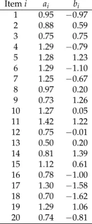
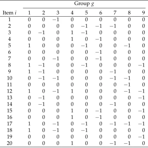
In TableA1, common item parameters (i.e., item loadings and item difficulties) are shown. Tables A2andA3show the values of the DIF indicator variableZigfor the condition of 10% and 30% biased items, respectively.

Table A1.Simulation Study: Common Item Loadings and Item Intercepts Itemi ai bi

1 0.95 −0.97

2 0.88 0.59

3 0.75 0.75

4 1.29 −0.79

5 1.28 1.23

6 1.29 −1.10 7 1.25 −0.67

8 0.97 0.20

9 0.73 1.26

10 1.27 0.05 11 1.42 1.22 12 0.75 −0.01 13 0.50 0.20 14 0.81 1.39 15 1.12 0.61 16 0.78 −1.00 17 1.30 −1.58 18 0.70 −1.62 19 1.29 1.06 20 0.74 −0.81

Table A2.DIF Indicator VariablesZigfor the Condition of 10% Biased Items Groupg

Itemi 1 2 3 4 5 6 7 8 9

1 0 0 0 0 0 0 0 0 0

2 0 0 0 0 −1 0 0 0 0

3 0 −1 0 0 0 0 0 0 0

4 0 0 0 0 0 0 0 0 0

5 0 0 −1 0 −1 0 0 0 0

6 1 0 0 1 0 0 0 0 0

7 0 0 0 0 0 −1 0 0 0

8 0 0 0 0 0 0 0 0 0

9 0 0 −1 0 0 0 0 0 0

10 0 0 0 0 0 0 0 0 0

11 0 0 0 0 0 0 0 0 0

12 0 0 0 0 0 0 0 0 0

13 0 −1 0 0 0 0 0 0 0

14 0 0 0 0 0 0 0 0 0

15 0 0 0 0 0 0 0 0 0

16 1 0 0 0 0 0 0 −1 0

17 0 0 0 0 0 −1 −1 0 0

18 0 0 0 1 0 0 0 −1 0

19 0 0 0 0 0 0 0 0 −1

20 0 0 0 0 0 0 −1 0 −1

Table A3.DIF Indicator VariablesZigfor the Condition of 30% Biased Items Groupg

Itemi 1 2 3 4 5 6 7 8 9

1 0 0 −1 0 0 0 0 0 0

2 0 0 0 0 −1 −1 −1 0 0

3 0 −1 0 1 −1 0 0 0 0

4 0 0 0 1 0 −1 0 0 0

5 1 0 0 0 −1 0 0 −1 0

6 0 0 0 0 0 −1 0 0 0

7 0 0 −1 0 0 −1 0 0 0

8 1 −1 0 0 −1 0 0 0 −1

9 1 −1 0 0 0 0 −1 0 0

10 0 −1 −1 0 0 0 −1 −1 0

11 0 0 0 0 0 0 0 −1 0

12 1 0 −1 1 0 0 0 −1 −1

13 0 −1 0 0 0 0 0 0 −1

14 0 −1 0 0 0 0 −1 0 0

15 0 0 0 1 0 −1 0 0 −1

16 0 0 0 1 0 −1 0 0 0

17 1 0 −1 0 −1 0 −1 −1 −1

18 1 0 −1 0 −1 0 0 0 0

19 0 0 0 0 0 0 0 0 −1

20 0 0 0 1 0 0 −1 −1 0

References

1. OECD.PISA 2015. Technical report; OECD: Paris, 2017.

2. Penfield, R.D.; Camilli, G. Differential item functioning and item bias. InHandbook of statistics, Vol. 26: Psychometrics; Rao, C.R.; Sinharay, S., Eds.; 2007; pp. 125–167. doi:10.1016/S0169-7161(06)26005-X. 3. Haebara, T. Equating logistic ability scales by a weighted least squares method. Jpn. Psychol. Res.1980,

4. Hu, H.; Rogers, W.T.; Vukmirovic, Z. Investigation of IRT-based equating methods in the presence of outlier common items. Appl. Psychol. Meas.2008,32, 311–333. doi:10.1177/0146621606292215.

5. Magis, D.; De Boeck, P. Identification of differential item functioning in multiple-group settings: A multivariate outlier detection approach. Multivar. Behav. Res. 2011, 46, 733–755. doi:10.1080/00273171.2011.606757.

6. Birnbaum, A. Some latent trait models and their use in inferring an examinee’s ability. InStatistical theories of mental test scores; Lord, F.M.; Novick, M.R., Eds.; MIT Press: Reading, MA, 1968; pp. 397–479.

7. Bechger, T.M.; Maris, G. A statistical test for differential item pair functioning. Psychometrika2015,

80, 317–340. doi:10.1007/s11336-014-9408-y.

8. Doebler, A. Looking at DIF from a new perspective: A structure-based approach acknowledging inherent indefinability. Appl. Psychol. Meas.2019,43, 303–321. doi:10.1177/0146621618795727.

9. Robitzsch, A.; Lüdtke, O. A review of different scaling approaches under full invariance, partial invariance, and noninvariance for cross-sectional country comparisons in large-scale assessments.Psych. Test Assess. Model.2020,62, 233–279.

10. Byrne, B.M.; Shavelson, R.J.; Muthén, B. Testing for the equivalence of factor covariance and mean structures: the issue of partial measurement invariance. Psychol. Bull. 1989, 105, 456–466. doi:10.1037/0033-2909.105.3.456.

11. von Davier, M.; Yamamoto, K.; Shin, H.J.; Chen, H.; Khorramdel, L.; Weeks, J.; Davis, S.; Kong, N.; Kandathil, M. Evaluating item response theory linking and model fit for data from PISA 2000–2012.Assess. Educ.2019,26, 466–488. doi:10.1080/0969594X.2019.1586642.

12. Kopf, J.; Zeileis, A.; Strobl, C. Anchor selection strategies for DIF analysis: Review, assessment, and new approaches. Educ. Psychol. Meas.2015,75, 22–56. doi:10.1177/0013164414529792.

13. Camilli, G. The case against item bias detection techniques based on internal criteria: Do item bias procedures obscure test fairness issues? InDifferential item functioning: Theory and practice; Holland, P.W.; Wainer, H., Eds.; Erlbaum: Hillsdale, NJ, 1993; pp. 397–417.

14. von Davier, A.A.; Carstensen, C.H.; von Davier, M. Linking competencies in educational settings

and measuring growth (Research Report No. RR-06-12). Educational Testing Service, 2006.

doi:10.1002/j.2333-8504.2006.tb02018.x.

15. González, J.; Wiberg, M. Applying test equating methods. Using R; Springer: New York, 2017. doi:10.1007/978-3-319-51824-4.

16. Kolen, M.J.; Brennan, R.L. Test equating, scaling, and linking; Springer: New York, 2014. doi:10.1007/978-1-4939-0317-7.

17. Lee, W.C.; Lee, G. IRT linking and equating. InThe Wiley handbook of psychometric testing: A multidisciplinary reference on survey, scale and test; Irwing, P.; Booth, T.; Hughes, D.J., Eds.; Wiley: New York, 2018; pp. 639–673. doi:10.1002/9781118489772.ch21.

18. Sansivieri, V.; Wiberg, M.; Matteucci, M. A review of test equating methods with a special focus on IRT-based approaches. Statistica2017,77, 329–352. doi:10.6092/issn.1973-2201/7066.

19. He, Y.; Cui, Z. Evaluating robust scale transformation methods with multiple outlying common items under IRT true score equating. Appl. Psychol. Meas.2020,44, 296–310. doi:10.1177/0146621619886050. 20. He, Y.; Cui, Z.; Osterlind, S.J. New robust scale transformation methods in the presence of outlying

common items. Appl. Psychol. Meas.2015,39, 613–626. doi:10.1177/0146621615587003.

21. Arai, S.; Mayekawa, S.i. A comparison of equating methods and linking designs for developing an item pool under item response theory.Behaviormetrika2011,38, 1–16. doi:10.2333/bhmk.38.1.

22. Battauz, M. Multiple equating of separate IRT calibrations. Psychometrika 2017, 82, 610–636. doi:10.1007/s11336-016-9517-x.

23. Kang, H.A.; Lu, Y.; Chang, H.H. IRT item parameter scaling for developing new item pools.Appl. Meas. Educ.2017,30, 1–15. doi:10.1080/08957347.2016.1243537.

24. R Core Team. R: A language and environment for statistical computing, 2020. Vienna, Austria. https://www.R-project.org/.

25. Robitzsch, A. sirt: Supplementary item response theory models, 2020. R package version 3.9-4. https://CRAN.R-project.org/package=sirt.

27. Stocking, M.L.; Lord, F.M. Developing a common metric in item response theory. Appl. Psychol. Meas. 1983,7, 201–210. doi:10.1177/014662168300700208.

28. Haberman, S.J. Linking parameter estimates derived from an item response model through separate calibrations

(Research Report No. RR-09-40). Educational Testing Service, 2009. doi:10.1002/j.2333-8504.2009.tb02197.x. 29. Muthén, B.; Asparouhov, T. IRT studies of many groups: The alignment method. Front. Psychol.2014,

5, 978. doi:10.3389/fpsyg.2014.00978.

30. Kim, S.H.; Cohen, A.S. A minimumχ2method for equating tests under the graded response model. Appl.

Psychol. Meas.1995,19, 167–176. doi:10.1177/014662169501900204.

31. Kim, S. An extension of least squares estimation of IRT linking coefficients for the graded response model.

Appl. Psychol. Meas.2010,34, 505–520. doi:10.1177/0146621609344847.

32. Pokropek, A.; Davidov, E.; Schmidt, P. A Monte Carlo simulation study to assess the appropriateness of traditional and newer approaches to test for measurement invariance. Struct. Equ. Modeling2019,

26, 724–744. doi:10.1080/10705511.2018.1561293.

33. Pokropek, A.; Lüdtke, O.; Robitzsch, A. An extension of the invariance alignment method for scale linking.

Psych. Test Assess. Model.2020,62, 303–334.

34. von Davier, M.; von Davier, A.A. A unified approach to IRT scale linking and scale transformations.

Methodology2007,3, 115–124. doi:10.1027/1614-2241.3.3.115.

35. Robitzsch, A.; Kiefer, T.; Wu, M. TAM: Test analysis modules, 2020. R package version 3.4-26. https://CRAN.R-project.org/package=TAM.

36. OECD.PISA 2006. Technical report; OECD: Paris, 2009.

37. Oliveri, M.E.; von Davier, M. Analyzing invariance of item parameters used to estimate trends in international large-scale assessments. InTest fairness in the new generation of large-scale assessment; Jiao, H.; Lissitz, R.W., Eds.; Information Age Publishing: New York, 2017; pp. 121–146.

38. Robitzsch, A.; Lüdtke, O. Linking errors in international large-scale assessments: Calculation of standard errors for trend estimation. Assess. Educ.2019,26, 444–465. doi:10.1080/0969594X.2018.1433633.

39. Robitzsch, A.; Lüdtke, O. Mean comparisons of many groups in the presence of DIF: An evaluation of linking and concurrent scaling approaches.OSF Preprints2020. doi:10.31219/osf.io/ce5sq.

40. Jerrim, J.; Parker, P.; Choi, A.; Chmielewski, A.K.; Sälzer, C.; Shure, N. How robust are cross-country comparisons of PISA scores to the scaling model used? Educ. Meas. 2018, 37, 28–39. doi:10.1111/emip.12211.

41. Robitzsch, A.; Lüdtke, O.; Goldhammer, F.; Kroehne, U.; Köller, O. Reanalysis of the German PISA data: A comparison of different approaches for trend estimation with a particular emphasis on mode effects. Front. Psychol.2020,11, 884. doi:10.3389/fpsyg.2020.00884.

42. DeMars, C.E. Alignment as an alternative to anchor purification in DIF analyses. Struct. Equ. Modeling 2020,27, 56–72. doi:10.1080/10705511.2019.1617151.

43. Finch, W.H. Detection of differential item functioning for more than two groups: A Monte Carlo comparison of methods. Appl. Meas. Educ.2016,29, 30–45. doi:10.1080/08957347.2015.1102916.

44. Andersson, B. Asymptotic variance of linking coefficient estimators for polytomous IRT models. Appl. Psychol. Meas.2018,42, 192–205. doi:10.1177/0146621617721249.

45. De Boeck, P. Random item IRT models.Psychometrika2008,73, 533–559. doi:10.1007/s11336-008-9092-x. 46. De Jong, M.G.; Steenkamp, J.B.E.M.; Fox, J.P. Relaxing measurement invariance in cross-national consumer

research using a hierarchical IRT model. J. Consum. Res.2007,34, 260–278. doi:10.1086/518532.

47. Fox, J.P.; Verhagen, A.J. Random item effects modeling for cross-national survey data. InCross-cultural analysis: Methods and applications; Davidov, E.; Schmidt, P.; Billiet, J., Eds.; Routledge: London, 2010; pp. 461–482.

48. Muthén, B.; Asparouhov, T. Recent methods for the study of measurement invariance with many groups: Alignment and random effects.Sociol. Methods Res.2018,47, 637–664. doi:10.1177/0049124117701488. 49. Pokropek, A.; Schmidt, P.; Davidov, E. Choosing priors in Bayesian measurement invariance modeling:

A Monte Carlo simulation study. Struct. Equ. Modeling 2020. Advance online publication, doi:10.1080/10705511.2019.1703708.

50. Asparouhov, T.; Muthén, B. Multiple-group factor analysis alignment. Struct. Equ. Modeling2014,

51. Barrett, M.D.; van der Linden, W.J. Estimating linking functions for response model parameters. J. Educ. Behav. Stat.2019,44, 180–209. doi:10.3102/1076998618808576.

52. Battauz, M. Factors affecting the variability of IRT equating coefficients. Stat. Neerl. 2015,69, 85–101. doi:10.1111/stan.12048.

53. Jewsbury, P.A.Error variance in common population linking bridge studies(Research Report No. RR-19-42). Educational Testing Service, 2019. doi:10.1002/ets2.12279.

54. Ogasawara, H. Standard errors of item response theory equating/linking by response function methods.

Appl. Psychol. Meas.2001,25, 53–67. doi:10.1177/01466216010251004.

55. Zhang, Z. Estimating standard errors of IRT true score equating coefficients using imputed item parameters.

J. Exp. Educ.2020. Advance online publication, doi:10.1080/00220973.2020.1751579.

56. Gebhardt, E.; Adams, R.J. The influence of equating methodology on reported trends in PISA. J. Appl. Meas.2007,8, 305–322.

57. Michaelides, M.P. A review of the effects on IRT item parameter estimates with a focus on misbehaving common items in test equating. Front. Psychol.2010,1, 167. doi:10.3389/fpsyg.2010.00167.

58. Monseur, C.; Berezner, A. The computation of equating errors in international surveys in education. J. Appl. Meas.2007,8, 323–335.

59. Sachse, K.A.; Roppelt, A.; Haag, N. A comparison of linking methods for estimating national trends in international comparative large-scale assessments in the presence of cross-national DIF. J. Educ. Meas. 2016,53, 152–171. doi:10.1111/jedm.12106.

60. Xu, X.; von Davier, M.Linking errors in trend estimation in large-scale surveys: A case study.(Research Report No. RR-10-10). Educational Testing Service, 2010. doi:10.1002/j.2333-8504.2010.tb02217.x.

61. Winter, S.D.; Depaoli, S. An illustration of Bayesian approximate measurement invariance with longitudinal data and a small sample size. Int. J. Behav. Dev. 2019. Advance online publication, doi:10.1177/0165025419880610.

62. Arce-Ferrer, A.J.; Bulut, O. Investigating separate and concurrent approaches for item parameter drift in 3PL item response theory equating. Int. J. Test.2017,17, 1–22. doi:10.1080/15305058.2016.1227825. 63. Fischer, L.; Gnambs, T.; Rohm, T.; Carstensen, C.H. Longitudinal linking of Rasch-model-scaled competence

tests in large-scale assessments: A comparison and evaluation of different linking methods and anchoring designs based on two tests on mathematical competence administered in grades 5 and 7. Psych. Test Assess. Model.2019,61, 37–64.

64. Han, K.T.; Wells, C.S.; Sireci, S.G. The impact of multidirectional item parameter drift on IRT scaling coefficients and proficiency estimates. Appl. Meas. Educ. 2012, 25, 97–117. doi:10.1080/08957347.2012.660000.

65. Huggins, A.C. The effect of differential item functioning in anchor items on population invariance of equating.Educ. Psychol. Meas.2014,74, 627–658. doi:10.1177/0013164413506222.

66. Lei, P.W.; Zhao, Y. Effects of vertical scaling methods on linear growth estimation. Appl. Psychol. Meas. 2012,36, 21–39. doi:10.1177/0146621611425171.

67. Pohl, S.; Haberkorn, K.; Carstensen, C.H. Measuring competencies across the lifespan-challenges of linking test scores. InDependent data in social sciences research; Stemmler, M.; von Eye, A.; W., W., Eds.; Springer: Cham, 2015; pp. 281–308. doi:10.1007/978-3-319-20585-4_12.

68. Tong, Y.; Kolen, M.J. Comparisons of methodologies and results in vertical scaling for educational achievement tests.Appl. Meas. Educ.2007,20, 227–253. doi:10.1080/08957340701301207.