Article
The Positioning of the Electromechanical System
Using Sliding Mode Control without a Reaching
Phase
Stefan Brock
Poznan University of Technology, Poland
* Correspondence: [email protected]; Tel.: +48-61-665-2627
Featured Application: The presented application is used in electromechanical tracking systems with precise control of position and speed.
Abstract: Precise and fast position tracking is essential for the correct operation of many industrial robots and CNC machine tools. This subject is also important in the control of the mount of the astronomical telescope, especially for the tracking of artificial satellites. As system parameters can change, a control method that is robust to changes in parameters must be used. Such a method is the sliding control, which, however, ensures the robustness only after reaching the sliding surface. Therefore, a new method was proposed in the paper, which eliminates the phase of reaching the sliding surface. The method consists of using a reference trajectory generator and determining the generalized error in relation to this trajectory. The procedure for designing the control system is presented. Next, the proposed method was verified on the laboratory stand. The described control method provides a robust system operation and can be easily implemented in the control system.
Keywords: sliding mode control; position tracking; reference signal generator; telescope mount; motion control; electrical drive;
1. Introduction
In the field of the robot manipulator and machine tool control, one of the important issues is the robustness of the servo drive system. Robustness is the ability of a closed-loop system to retain a specified dynamic performance despite plant modeling uncertainties and external disturbances. The robustness of the servo system applied to each joint of a manipulator or axis of the machine tool enables no interferences among other servo drives.
Many applications require operation under dynamically changing conditions regarding the reference position. Such changes in target position either due to the physical movement of the target or due to additional sensor information provided during the motion require on-line updating of the reference trajectory. Furthermore, in direct drive, it is very important to obtain trajectory for smooth motion (i.e. no discontinuity at least in velocity and acceleration) under constraints of maximum limiting values of velocity, acceleration and jerk at the same time. This requires an on-line re-programming of the reference-trajectory based on the current position, velocity, acceleration and jerk without an abrupt change of them. In the paper new concept of reference trajectory generator is proposed.
Astronomical telescope mounts are electromechanical systems with very high demands on motion control precision. A special case is the observation of artificial satellites of the Earth. In the Low Earth Orbits rang (LEO, 160-2000 km), where the angular speed of the satellites are significant (up to 2 deg/s), the precision tracking is an open problem.
Sliding mode controllers are well known to be robust against bounded, unstructured modeling errors and external disturbances. However, it also introduces actuator chattering phenomena that should be avoided in many physical systems, such as servo control systems, structure vibration control systems and robotic systems. This subject is considered in many works and is omitted here [1-3]. The discontinuous switching function has been replaced by a continuous approximation.
Basically, the sliding mode control motion has two phases, i.e., the reaching phase and the sliding phase. The robustness is guaranteed only after the system reaches the switching surface. Therefore, the system is sensitive to parameter uncertainty and disturbance in the reaching phase.
An approach to reduce the effect of reaching phase dynamics on control performance is to make the sliding mode occur from the beginning of the movement.
To overcome this
problem
, a sliding mode control law based on a time-varying switching line is proposed in many papers. Section 2 briefly describes the application of the sliding mode control method to an electromechanical system of unknown parameters. A systematic approach to reducing the effect of reaching phase, based on the minimization of selected quality objectives is presented in work [4]. This method is briefly described in section 3. Section 4 of this paper is devoted to a new method, in which the reference signal generator, presented short earlier in [2], was applied. The laboratory testing stand is described in section 5.1, while the results, discussion, and concluding remarks are presented in section 5.2.2. Classical Sliding Mode Control Law with Reaching Phase
Given a class of SISO dynamic system described by the equation:
( , )
( , )
( , )
n n
d x
f
t
b
t u
d
t
dt
x
x
x
(1)
for which a
referencestate vector
and
state vector
are defined as:
1 ref 1 ref
ref ref
1
1
T T
n n
n n
dx
d
x
dx
d
x
x
x
dt
dt
dt
dt
x
K
x
K
(2)
The
f
( ), ( ), ( )
b
d
functions describe respectively the object's own dynamics, input signal path, and external interference. The tracking error vector of the reference value is proposed as:1 ref 1 T n n
de
d
e
e
dt
dt
e = x - x
K
(3)
In the
space
of error is defined sliding surface
( )
t
1 1 1
1 0 1 2 1 1 2
1
( , )
(
1)
0
n n n k
k n k k n n n n n
n
d
d
e
t
e
k
dt
dt
d
e
d
e
n
e
dt
dt
e
L
(4)
Coefficient λ is selected in the design of control law. It is a Lyapunov function in the form:
2
1
( , )
( , )
2
V
e
t
e
t
(5)
The condition for the stability of the control system is:
2
( , )
1
( , )
( , )
0
2
dV
t
d
t
t
dt
dt
e
The state vector must reach the surface
( )
t
in a finite time and then stay on the surface. In the first control law design stage, it is assumed that it is precisely known the controlled system (1), namely:f
(
x
,
t
)
f
(
x
,
t
),
b
(
x
,
t
)
b
(
x
,
t
),
d
(
x
,
t
)
0
(7)
where
f
ˆ( )
andb
ˆ( )
are respectively estimates of the real functionsf
( )
andb
( )
. In this case, a compensating control law can be so designed (8) that guarantees the fulfillment of the condition (6) and correct operation of the system.ref 1 1
1
1
d
d
ˆ
( , )
( , )
d
d
n n n k
k
n n k
k
n
x
e
u
b
t
f
t
k
t
t
x
x
(8)
In the real case only ranges of the variability of object (1) parameters are known:
min max
0
b
b
( , )
x
t
b
(9)
min
( , )
maxf
f
x
t
f
(10)
( , )
d
x
t
D
(11)
In this case, it is necessary to extend the control law by adding the switching term:
1
ˆ
ˆ
( , )
sgn( )
u
u
b
x
t
K
(12)
wherein the coefficient K is selected so as to ensure the condition (6) in each case.Figure 1 shows the block diagram of the electromechanical control system. The control problem is to get the position output
to achieve the desired position
setasymptotically in the presence of the nonlinear disturbances. The control system includes an internal torque control loop and an external speed and position control layer. The internal layer depends on the type of drive used. In the case of a popular PMSM drive [5, 6, 7], it will usually be a vector control, keeping the d current component equal to 0. The reference value of the q component of the current is supplied from the outer layer. The outer layer is universal and does not depend on the type of electric drive.
PWM Inverter
PMSM
Enc
Position and speed controller
s
Torque controller
set
, ,
a b c
i i i s
-
Figure 1. Block diagram of the electromechanical control system. The equation describes the mechanical model of the drive system:
2
ref 2
d 1 d d
sgn
d d d
T
c g T
k
d T T i
t J t t J
(13)
where
J
is the moment of inertia in respect of the motor shaft,k
T is the motor torque coefficientis the coefficient of viscous friction and
T
c is the Coulombic torque. For a wide class of drives canspecify the current component iT forming the torque. In the case of a surface magnet PMSM drive
with vector control, the q component of the current vector
i
q is proportional to the generated motortorque. Taking into account the fast current control loop, its internal dynamics can be neglect
ref
T T
i i
(14)
The reference signal of the current ref
T
i is the output of the sliding mode controller.
2
2
d
d
d
t
d
t
(15)
ref d
d
e e
t
(16)
Switching surface
( )
t
is a line, and for reference step change it is defined as:d
0
0
d
e
e
t
(17)
where
describes the slope of the line on the state phase plane. The control law for reference step change is design as:ref 1 ˆ d ˆ d
ˆ
d d
T T
e e
i d J
k t t
(18)
ref ˆrefsgn
T T
i i K
(19)
The current reference consists of two components: equivalent control ˆref
T
i , which compensates the known part of an object and component iTs K sgn
, ensuring a sliding motion. The sliding mode will be maintained if, at any time, the current reference value does not exceed the permissive limitI
max.ref max
T
i I
(20)
To eliminate the chattering phenomena, the switching term is replaced by its continuous approximation:
ref ref ref ?ref max
sgn( ) sat( , )
s
T T T T s T s
i i i i K
i K
(21)
The sat( ) function is continuous and determined by the width of the approximation zonemax
0
max max
max
max
for sat( , )
sgn( ) for
.
(22)
In the reaching phase, the system with the maximum possible current aims to achieve the switching surface. During the sliding phase, motion occurs on the switching line described by
0 , and the dynamics of movement depends only on the coefficient
.3. Sliding Mode Control Law based on a Time-Varying Switching Line
additional variable offset, and figure 2b shows a line with a variable slope coefficient. The first option was chosen as a reference to implementation.
e
d d
e t
0 tt
end tt
(a)
e
d d
e t
0 tt
end tt
(b)
Figure 2. Time-varying switching line: (a) with additional variable offset; (b) with a variable slope coefficient.
The following modification of the generalized equation error is used:
d d e
e A B t
t
,
(23)
where A is the initial offset, and B is the speed of switching line run, respectively. Described in this way switching line moves in the state space, as shown in figure 2a. The starting position is selected so that the point corresponding to an initial error (in the time of setpoint position step change) was on the switching line. While moving the sliding line at speed B, the control law should be modified to form:
ref 1 ˆ d ˆ d
ˆ
d d
T T
e e
i d J B
k t t
,
(24)
Coefficient B must be so selected as to satisfy condition (20). The considered line stops moving at the time
t
end, when the trajectory reaches the sliding line passing through the origin, and afterwards,equation (18) applies. Constants A is calculated based on reference signal value. For that purpose, the integral of the absolute error (IAE) is minimized subject to the input signal and velocity constraints [4]. Constants A, B and time tend at which the control system switch to the fixed line (5) need to be
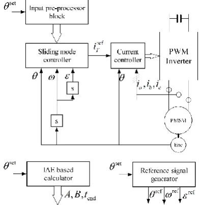
calculated before the motion start. The structure of such a control system is shown in Figure 3, where Input pre-processor block is replaced by IAE based calculator block.
4. Sliding mode control with reference signal generator
The structure presented in Chapter 3 has a significant disadvantage. The IAE calculations are performed off-line before the start of the movement. If, on the other hand, a change in the reference value can occur during the movement, it is necessary to use much more complex calculation algorithms. Therefore, a new, modified structure is proposed, working online without the need for recalculation. In this case, block Input pre-processor block in Figure 3 is replaced by the block Reference signal generator.
4.1. The Classic Reference Signal Generator
A classical approach to solving the trajectory generation problem online would be to solve an optimal control problem in real-time [8]. The standard indirect and direct methods for the numerical solution of optimal control problems can be found in many papers. These methods generally run as a command pre-processor and are relatively slow. The block diagram of such a generator is shown in Figure 4. Time-optimal control with a limit of a jerk (a derivative of acceleration) is assumed. The position error is used to determine the fixed value of the permissible jerk intervals. The jerk signal is then integrated one after the other and the reference acceleration, the reference speed and the reference position for the control system are calculated respectively. Additional feedback compensates for numerical integration errors.
-+
ref
ref
ref
set
Interwal choice
max
max
s
1
max
s
1
s
1
Figure 4. Block diagram of the referce signal generator with interwal choice. . 4.2. The Proposed Reference Signal Generator
The structure of the generator based on an idealized model of the drive control system is proposed (fig. 5). Drive is modeled as two integrators with a delay corresponding to the current control loop. The linear integral controller for acceleration and proportional controller for speed are used. The nonlinear position controller has the square root characteristics with the limitation of maximum speed and acceleration. Such a system does not require any off-line calculations, it can process both the step input signal and free continuous signal without any modifications. The acceleration limiter is selected so as to ensure that the limitation current is not exceeded over the whole range of drive operation. In this case, the true drive can follow the reference trajectory accurately.
k k
1
z
k
z
1
z
1 s
1
s
1
z
-+ +
-+ +
- + +
+
+
+ ref
ref
ref
set
Nonlinear position controller with acceleration limit
Speed P controller
Acceleration I controller with limit
Model of current
control loop Model of ideal mechanical subsystem
t
Figure 5. Block diagram of the proposed reference signal generator.
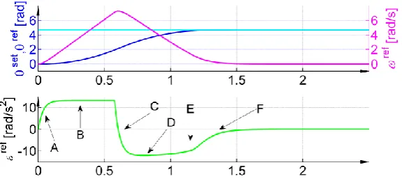
Figure 6. Example of a reference trajectory after an input signal step-change. 4.3. The Sliding Mode Control with Reference Signal Generator
Command position input signal
set is processed by reference signal generator to the reference position
ref, velocity
refand acceleration
ref. The generalised error is redefined as:ref ref
d d
, ,
d d
e e
e e
t t
(25)
Since the reference signals change continuously, with dynamics corresponding to the worst-case motor load case (with maximum load torque, over the full range of moment of inertia variations), there is no reaching phase during system operation. Therefore, the sliding mpde control system can be designed as described in Chapter 2. In addition, speed and acceleration reference signals are available, allowing a simple creation of a compensation component for the control law.
5. Experimental Results
5.1. Laboratory Stands
To verify the effectiveness of the proposed low-speed estimation methods, laboratory tests were also carried out. Primarily experiments were carried out using robotic telescope mount developed at Poznan University of Technology [9]. The plant consists of a robotic mount and an astronomic telescope with a mirror of diameter 0.5 m. The robotic mount alone includes two axes driven independently by 24 V permanent magnet synchronous motors (PMSM). Control algorithms have been implemented in C++ using a processor with ARM Cortex-A9 core clocked at 600 MHz. The mechanical structure of the laboratory stand is shown in Figure 7a. In order to obtain a wider range of parameter variability under laboratory conditions, the final tests were carried out on a direct drive PMSM test bench with a large range of load changes (Figure 7b).
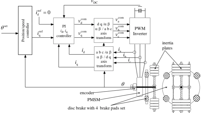
Figure 8 presents the structure of the laboratory stand. The system consists of three main parts: the motor with load construction, a PWM converter and the control algorithm implemented in the controller [10]. A set of metal plates (4) fixed to the arm (6) mounted on the motor shaft (8) enables us to vary the moment of inertia. The disc brake (7) with four adjustable brake pads (5) is fixed to the motor shaft. This adjustable brake can be used to model dry friction, typically for many machining processes.
(a) (b)
Figure 7. Laboratory stands used for testing: (a) robotic telescope mount (in this configuration with an 11-inch diameter mirror telescope); (b) direct drive with high load variation.
P
o
si
ti
o
n
/s
p
eed
c
o
n
tr
o
ll
er
set
ref q i
PI
id,iq controller 0
ref d i
d q /
/ a b c axis transform com
q v
com d v
PWM Inverter
{
a b c /
/ d q axis transform d
i
q i
com a v
com b v
com c v
a i
b i
c i
DC v
encoder PMSM
disc brake with 4 brake pads set
inertia plates
Figure 8. Block diagram of laboratory stand with and vector controlled PMSM direct drive. 5.2. Experimental Results
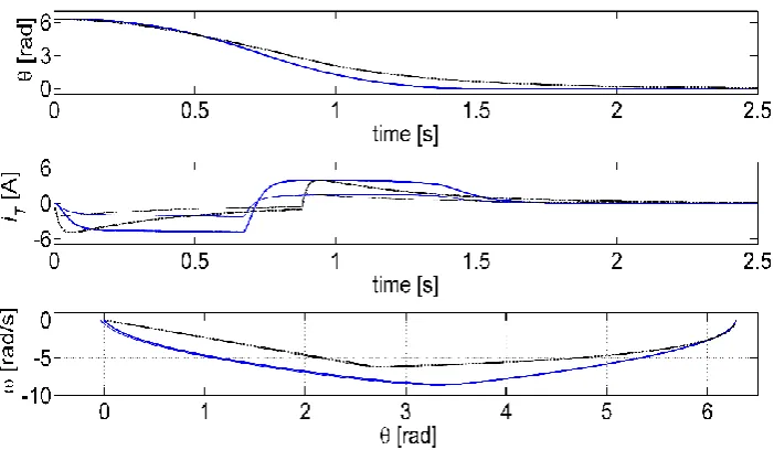
The correctness of the proposed control approach was evaluated and a number of tests were carried out for different operating conditions. Only selected, representative results were included in the paper. Figure 9 shows the recorded waveforms for the sliding control algorithm with an reaching phase. In the figure, the position, current versus time and speed versus position are shown from above. A thin line corresponds to the load case with the smallest inertia (without load plates), a thick line corresponds to the load case with the greatest inertia (with a set of inertia plates). The movement starts from the phase of reaching the sliding line. During the access phase the drive operates with a maximum current of 6 A. In this phase, the movement is dependent on the load. After the access phase, the movement takes place along the sliding trajectory, represented by a straight line.
thanks to the proposed reference trajectory generator with an square root position controller and acceleration limitation, the waveforms are significantly faster. At the same time, the current limitation is kept within the entire operating range. This is fully consistent with the approved design objectives. In conclusion, it can therefore be considered that the proposed control structure with a reference generator can be recommended for robust servo drive control applications.
Figure 9. Sliding mode control with reaching phase. Thick line - maximum load, thin line - minimum load.
Figure 10. Sliding mode control with reaching phase. Thick lines - maximum load, thin lines - minimum load. Black lines - control from chapter 3, blue lines - control from chapter 4.
Funding: This work was supported by the National Science Centre (NCN) under the grant No 2014/15/B/ST7/00429, contract No UMO-2014/15/B/ST7/ 00429.
Conflicts of Interest: The author declare no conflict of interest. The funders had no role in the design of the study; in the collection, analyses, or interpretation of data; in the writing of the manuscript, or in the decision to publish the results.
1. Sabanovic, A., Variable Structure Systems With Sliding Modes in Motion Control - A Survey, IEEE Transac-tions on Industrial Informatics, vol. 7, no. 2, pp. 212–223, May 2011.
2. Brock, S.: Robust position control for direct drive by integral sliding mode controller with reference trajectory generator, Symposium on Electromagnetic Phenomena in Nonlinear Circuits, Pula, Croatia, 2012,.
3. Utkin, V., Gulder, J., and. Shijun M, Sliding Mode Control in Electro-mechanical Systems, CRC Press, 1999.
4. Bartoszewicz, A. and Nowacka-Leverton, A.: Time-Varying Sliding Modes for Second and Third Order Sys-tems, Springer, 2009.
5. Wang, D.; Yuan, T.; Wang, X.; Wang, X.; Wang, S.; Ni, Y. Performance Improvement for PMSM Driven by DTC Based on Discrete Duty Ratio Determination Method. Appl. Sci.2019, 9, 2924.
6. Pietrusewicz, K.; Waszczuk, P.; Kubicki, M. MFC/IMC Control Algorithm for Reduction of Load Torque Disturbance in PMSM Servo Drive Systems. Appl. Sci.2019, 9, 86.
7. S.; Brock, D.V. Lukichev and G. L. Demidova, "Minimizing torque ripple in PMSM drive-by cuckoo search algorithm," 2017 19th European Conference on Power Electronics and Applications (EPE'17 ECCE Europe), Warsaw, 2017, pp. P.1-P.9.
8. Pietrusewicz, K.; Waszczuk, P.; Kubicki, M. MC_MoveAbsolute() 4th Order Real-Time Trajectory Generation Function Algorithm and Implementation. Appl. Sci.2019, 9, 538.
9. S.; Brock, D.; Łuczak, K.; Nowopolski, T. Pajchrowski, and K. Zawirski, "Two Approaches to Speed Control for Multi-Mass System With Variable Mechanical Parameters," in IEEE Transactions on Industrial Electronics, vol. 64, no. 4, pp. 3338-3347, April 2017.