Article 1
Spatial Pattern Dynamics Analysis at Coastal Area
2Using Spatial Metric in Pekalongan, Indonesia
3Ali Wijaya 1,*, Cahyono Susetyo 1, Azillatin Q. Diny 1, Danika H. Nabila 1, Rahel P. Pamungkas 1,
4
Mohammad Hadikunnuha 2, and Nursakti Adhi Pratomoatmojo 1
5
1 Department of Urban and Regional Planning, Institut Teknologi Sepuluh Nopember, Surabaya 60111,
6
Indonesia; [email protected] 7
2 Department of Geomatic Engineering, Institut Teknologi Sepuluh Nopember, Surabaya 60111, Indonesia;
8
* Correspondence: [email protected]; Tel.: +63-857-498-26432 10
11 12
Abstract: Pekalongan is one of several cities that lies in the northern coast of Java island which is 13
often flooded due to sea level rise. This condition impacted its urban development characteristic 14
and increase in the future. In this research both Geographical Information System based and Spatial 15
Metric approach are used. The spatial pattern is analyzed by using spatial metric based on the 16
exploration of land use change that occurred. In this research, the spatial pattern is focused on 17
aggregation pattern and diversity in coastal area. The result shows that the land use of coastal area 18
are dominated with swamp, then followed by settlement and fishpond. It is also shown that the 19
greatest land use change occurred on paddy field and swamp areas. Based on the spatial metric 20
calculation, the aggregation level of land use decrease periodically and has a small growth level. It 21
is indicated from its metric value aggregation and diversity from two periods: 2003-2009 and 2009-22
2016. Overall the land use of Pekalongan experienced large dynamics, especially in its coastal area. 23
The spatial pattern trend in those area tend to be more sprawl as defined by the decrease of 24
aggregation pattern and low level of land use growth pattern. 25
Keywords: : Spatial Pattern; Land Use; Spatial Metric; Aggregation; Diversity 26
27
1. Introduction 28
Spatial element is something that must be considered in every region’s development planning. 29
Spatial information shows the function of a location or a region. The usage of spatial analysis has 30
been developed for locational based analysis by using GIS (Geographical Information System). One 31
of many output that can be used as a consideration material in policy decision making is spatial 32
model. The computer-based model of land use change and urban growth has become an important 33
tool to support regional planning [1][2]. One process that indicates the development of a region is the 34
change of land use which is dynamic and can be observed with multi-temporal spatial analysis. Both 35
regional and urban planning always receive great attention in recent decades, especially the ability 36
to form landscape constantly [3][4]. The complexity and urban development can be characterized by 37
the complexity of spatial patterns and land use. Spatial vision area is always directed by the shape 38
and spatial distribution that is ideal for its landscape [5] and to understand it spatial analysis is 39
needed. 40
Spatial metric has been known as a spatial analysis which is related with the spatial development 41
in urban area. It is defined as a measurement which is derived from digital-based thematic map 42
analysis that shows the spatial heterogeneity at certain scale and resolution [2]. Spatial metric is also 43
known as a quantitative approach that can be used to assess spatial characteristic of land use and 44
urban structure. When spatial metric is being used for multi temporal, it could describe the level of 45
to interpret spatial pattern in land use change since it could provide additional information about the 47
structure of change ad could be continued with land use change modelling [7]. As a result, the spatial 48
pattern that are derived from the interpretation of spatial metric, such as density pattern and 49
accretion of land use, shows the development level of an area which led to the urgency to the usage 50
of spatial analysis. 51
Pekalongan is a city in Central Java Province Indonesia which is located in the northern coast of 52
Java Island. Tidal flood has become an important issues since it is often occurred in this city as a result 53
of sea level rise [8][9][10][11][12]. Tidal flood is the most serious threat from sea level rise that can 54
only be reduced impact [13]. Because of this phenomenon, the land use change in Pekalongan has 55
been also affected [14]. Land use change in a landscape is driven by driving force factors [15][16]such 56
as sea level rise in Pekalongan. Even though, in general, the land use of Pekalongan has not been 57
affected, shifts in function and usage of land have been identified, e.g. land use for paddy field has 58
been decreasing significantly [17]. Thus, it indicates that productive land has been dominating the 59
shift of function since one of land’s characteristics is vulnerable of natural phenomenon such as sea 60
level rise [18]. If it is associated with the trend of climate change, the impact of sea level rise will be 61
even greater [19] including in Pekalongan [20]. Based on the previous study [21], the tidal flood model 62
of Pekalongan has predicted that 50,68% of the whole area will be flooded by the year 2030. Tidal 63
flood has been also noticed as one of several factors that caused the land use change of Pekalongan 64
during 2003-2009 [21].This condition led to a fragmentation pattern and non-optimum mixed land 65
use which are Pekalongan’s development characteristics. Therefore, the accuracy of land use and its 66
management in Pekalongan has become an urgency to be considered in planning process [22] to 67
minimize the risk from natural disaster, such as tidal flood [10]. Thus, regarding this situation an 68
analysis on land use change and spatial pattern by using spatial approach is needed in order to 69
understand and optimize the development of Pekalongan. 70
2. Materials and Methods 71
2.1 Study Area 72
This research took place in the coastal area of Pekalongan, which geographically lays between 73
6o50'42"-6o55'44" LS and 109o37'55 "-109o42'19" BT. Located in the province of Central Java Indonesia,
74
Pekalongan has a total area of 4,525 hectares, or about 0.14% of the area of Central Java Province. 75
Administratively, Pekalongan is consisted of 4 districts, with 1 district in coastal area. The coastal 76
district itself is consisted of 7 villages [23]. According to its elevation, Pekalongan is classified as a 77
lowland area: 1 meter of land between the region of the north to the highest 6 meters above sea level 78
in the southern region. The average slope percentage is between 0-5% which is considered relatively 79
flat. Physically, Pekalongan is considered as a city which is prone to disasters, such as tidal flood. The 80
tidal flood in Pekalongan occurred almost every day when the tide is going high [14] . This 81
phenomenon led to infrastructure damages and also impacted social and economic life of local 82
communities. Above all, the existing land use of Pekalongan is the most impacted aspect. 83
84
Figure 1. Location of the study area in Pekalongan, Indonesia 85
Study area is on North Pekalongan which is a coastal area directly adjacent to the sea. All areas 86
rise. Each village area in North Pekalongan is an area affected by sea level rise. Here for the village 88
in the study area. 89
Table 1. Villages administration in North Pekalongan 90
VILLAGES AREA (Ha) PERCENTAGE (%)
Bandengan 193.53 12.57
Degayu 400.86 26.04
Kandang Panjang 182.10 11.83
Krapyak 358.38 23.28
Padukuhan Kraton 137.66 8.94
Panjang Baru 132.32 8.59
Panjang Wetan 134.67 8.75
TOTAL 1539.53 100.00
2.2 Data 91
In this study, the required data is geospatial data in Pekalongan with multi-temporal 92
dimensions. Data that used focused on the aim to determine the spatial pattern of land use in the 93
coastal area of Pekalongan. Land use data were obtained from high resolution Digital Globe's 94
Quickbird imageries with acquisition date at 2003, 2009, and 2016. Then the phenomenon of tidal 95
flood as the driving factor of land use change was observed directly with the primary survey. Data 96
and sources used can be seen in the following table. 97
Table 2. A set of geospatial data and source 98
DATA SOURCE OF DATA DATE
Administrative Boundary Map Statistics of Pekalongan 2003, 2009, 2016 Sattelite Imageries Pekalongan Digital Globe’s Quickbird 2003, 2009, 2016 Digital Elevation Model Topographic Map of Indonesia (RBI) 2001
Tidal flood Primary survey 2016
2.3 Land Use Change Mapping 99
This process itself require land use data from different time dimension (multi-temporal), which 100
are data from 2003, 2009, and 2016 that were obtained from Quickbird imageries interpretation which 101
were classified into different land use types, based on its homogenous appearance, by using 102
Geographical Information System (GIS). Quickbird imageries that has been set for the coordinate 103
system can be manually delineated land use with the visual interpretation techniques [24] based on 104
their characteristics. Classification of land use in this study is more directed at supervised 105
classification. After this step is done, the next step is validation which is done through ground 106
checking. The ground checking step is then followed with a process that compares the land use 107
change from 3 periods (2003, 2009, and 2016) through overlay analysis. The result of land use change 108
mapping analysis is showing the dynamics of land change in coastal area of Pekalongan which is 109
characteristic of flooded area of sea level rise. 110
2.4 Spatial Patterns Analysis of Land Use by Spatial Metric 111
This analysis proceed the result from land use change mapping by using a method called spatial 112
metric resulting spatial pattern of Pekalongan coastal area’s land use . Spatial metric itself is a method 113
that allows user to formulate metrics-based dynamic spatial pattern. The spatial pattern dynamics of 114
land use that are identified in a multi temporal manner are spatial patterns in the period 2003-2009 115
and 2009-2016. In this study, the analysis process is conducted by using the ArcGIS 10.4 software, 116
combined with Fragstats 4.2 [25]. The output of this analysis are calculation result and chart, which 117
aspect and spatial pattern such as fragmentation and diversity pattern. Fragmentation pattern 119
indicates aggregation level of land use, will know the trend of density value in coastal area of 120
Pekalongan. Then diversity pattern will indicate the level of land use growth of the tendency of 121
diversity value in each period. From these results will be identified spatial patterns of the landscape 122
as a whole on the coastal area of Pekalongan. 123
2.5 Selection of Metrics 124
Spatial pattern is something that shows the placement or arrangement of objects on the surface 125
of the earth [26]. The spatial pattern in this study focuses on multi-temporal patterns of fragmentation 126
and diversity in landscape level (coastal area of Pekalongan). It is used as a variable to analyze the 127
spatial pattern based on the fragmentation and diversity categories [27] which is adjusted based on 128
the purpose of this research and calculated with the tools from Fragstats. The type metric is as follow: 129
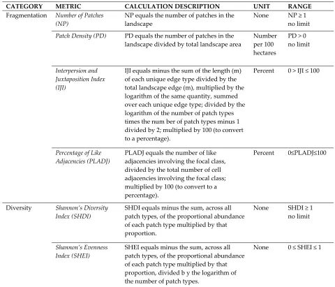
Table 3. The type of metrics used 130
CATEGORY METRIC CALCULATION DESCRIPTION UNIT RANGE
Fragmentation Number of Patches
(NP)
NP equals the number of patches in the landscape
None NP ≥ 1
no limit
Patch Density (PD) PD equals the number of patches in the landscape divided by total landscape area
Number per 100 hectares
PD > 0 no limit
Interpersion and Juxtaposition Index (IJI)
IJI equals minus the sum of the length (m) of each unique edge type divided by the total landscape edge (m), multiplied by the logarithm of the same quantity, summed over each unique edge type; divided by the logarithm of the number of patch types times the num ber of patch types minus 1 divided by 2; multiplied by 100 (to convert to a percentage).
Percent 0 > IJI ≤ 100
Percentage of Like Adjacencies (PLADJ)
PLADJ equals the number of like adjacencies involving the focal class, divided by the total number of cell adjacencies involving the focal class; multiplied by 100 (to convert to a percentage).
Percent 0≤PLADJ≤100
Diversity Shannon’s Diversity
Index (SHDI)
SHDI equals minus the sum, across all patch types, of the proportional abundance of each patch type multiplied by that proportion.
None SHDI ≥ 1
no limit
Shannon’s Evenness Index (SHEI)
SHEI equals minus the sum, across all patch types, of the proportional abundance of each patch type multiplied by that proportion, divided b y the logarithm of the number of patch types.
None 0 ≤ SHEI ≤ 1
Each metric has its own formula and interpretation. The formula of each type of metric is a way 131
to identify the spatial pattern in the accordance with the function of the metric itself. For the 132
algorithm’s calculation in each metric, sourced from McGarigal et al [28]. The results of the spatial 133
analysis of this metric in the form of statistical calculations that can be used as a comparison chart of 134
spatial patterns of land use 135
3.1. Spatio-Temporal Landuse Mapping 137
Land use mapping is used to determine the spatio temporal dynamics of land use that is 138
occurred. Land use map in this study used the interpretation of the Quickbird satellite imageries on 139
2003, 2009, and 2016. Quickbird imageries has resolution up to 0,6 m, the imagery provides detail 140
resolution and fits with the needs of this research. The process of land use classification of the image 141
in this study using a digitation on screen with GIS based on the visual interpretation of the satellite 142
imagery to be the land use class vector. From the type of land use classification and the characteristics 143
of each type of land use that could be identified, digitization has been done with a depth of 1: 10000 144
scale to become raster data with 5M resolution. The use of 5x5 meter resolution takes into account to 145
the level of detailed land use and already covers the smallest land use area in the study area. Land 146
use maps from previous period are adapted from a previous study in Pekalongan [21] and interviews 147
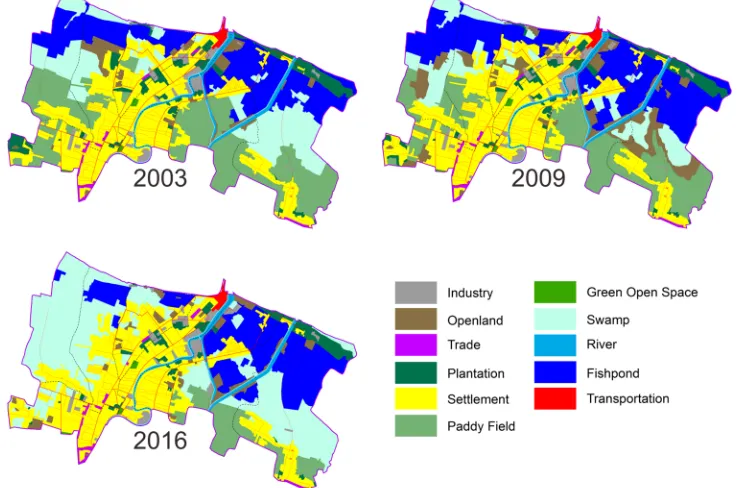
with local inhabitants. Below is a map of multi-temporal land use in the coastal area of Pekalongan 148
149
Figure 2. Multi-temporal land use map of study area 150
The map above shows the dynamics of land use. Changes in the area of multi temporal land use 151
show the characteristics of Pekalongan’s coastal area, which has the driving force in the form sea level 152
rise. The statistics changes of the coastal area’s land use could be seen as follow: 153
Table 4. Statistics of land use area in study area 154
LAND USE CLASS LAND USE AREA (Ha) LAND USE CHANGE (Ha)
2003 2009 2016 2003-2009 2009-2016 2003-2016
Industry 35.00 38.31 42.29 3.31 3.98 7.29
Openland 51.13 126.25 50.13 75.12 -76.11 -0.99
Trade 10.91 11.13 12.21 0.21 1.08 1.29
Plantation 83.49 69.33 58.15 -14.17 -11.17 -25.34
Settlement 419.66 450.30 469.86 30.64 19.56 50.20
Paddy Field 351.06 281.97 95.96 -69.10 -186.00 -255.10
Swamp 252.84 163.01 484.29 -89.83 321.29 231.46
Green Open Space 3.21 3.21 3.21 0.00 0.00 0.00
River 40.30 40.30 40.30 0.00 0.00 0.00
LAND USE CLASS LAND USE AREA (Ha) LAND USE CHANGE (Ha)
2003 2009 2016 2003-2009 2009-2016 2003-2016
Transportation 7.67 7.67 7.67 0.00 0.00 0.00
From the statistics it could be inferred that Pekalongan’s coastal area experienced such dynamic 155
significant changes. The most dominant land use in 2016 in North Pekalongan is swamp area, which 156
increased rapidly compared to the previous period, which reach 321,29 Ha. The widespread 157
characteristic of swamps in coastal areas of Pekalongan indicates the dominant impact of sea level 158
rise. The second largest land use is settlement area, which increased on each period but it tends to be 159
small for the addition of breadth. Thirdly, there is paddy field, which decreased significantly. From 160
2003 to 2006, the wide of agricultural land in coastal area of Pekalongan has reduced by 255, 10 Ha 161
due to its water imundation from sea level rise. So that from the dynamics of land use in Pekalongan’s 162
coastal area it could be inferred that the formed spatial pattern is related with the tendency level of 163
fragmentation and diversity in Pekalongan’s coastal area. 164
3.2 Aggregation Pattern Metric 165
Spatial patterns which analyzed for dynamics include spatial land use aggregation that is 166
calculated in landscape level. Metric aggregation calculation also used the multi temporal land use 167
data in the form of raster. The level of land use density in coastal area of Pekalongan has its own 168
characteristic due to the phenomenon of tidal flood from sea level rise that occured. This is a driving 169
factor for changes in land use that will certainly affect the level of urban aggregation form. The 170
simulation result shows the calculation of metric for each year and will know the dynamics of spatial 171
pattern of land use density. 172
173
(a) (b)
174
175
(c) (d)
176
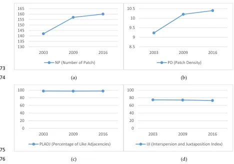
Figure 3. Aggregation pattern metric dynamics in landscape, (a) Number of Patch, (b) Patch Density, 177
(c) Percentage of Like Adjacencies, (d) Interspersion and Juxtaposition Index 178
From the results of these calculations, it can be known for dynamic patterns of aggregation in 179
the period 2003, 2009, and 2016 in Pekalongan coastal region that includes NP, PD, PLADJ, and IJI. 180
130 135 140 145 150 155 160 165
2003 2009 2016
NP (Number of Patch)
8.5 9 9.5 10 10.5
2003 2009 2016
PD (Patch Density)
0 20 40 60 80 100
2003 2009 2016
PLADJ (Percentage of Like Adjacencies)
0 20 40 60 80 100
2003 2009 2016
The value of NP in the coastal areas of Pekalongan in every period always increases the patch with 181
total in the period 2003-2016 added until 18 patches. Number of Patch (NP) is a metric measurement 182
of spatial density patterns which calculated from the number of patches. The greater of NP value, 183
indicating the greater of the fragmentation of the type of use that occurs. The PD value of statistic is 184
equal to the NP, increasing the patch density value for each period. PD in 2003 has a value of 9.23 185
patch/100ha to 10.4 patch/100ha in 2016. PD is a metric that measures the density and level of 186
fragmentation of land use or the area scope of the patch density. The bigger PD value, the less spatial 187
density of land use. Then the value of PLADJ in each period tend to be static and experience to the 188
dynamics of a very small value that is under 1%. PLADJ is a metric of measurement for the level of 189
patch type aggregation on each type of land use which shows the percentage of cohesiveness of land 190
use. Furthermore, the value of IJI shows a decrease in value, but relatively small. For the reduction 191
of IJI value for the period 2003-2016 is under 2%. IJI is the calculation of the dispersed index value of 192
land use in a landscape. 193
The coastal area of Pekalongan has characteristics in accordance with the dynamics of metric 194
aggregation values that have been analyzed. Furthermore, each village area in Pekalongan’s coastal 195
area will have its own characteristics which then form an area and affect to composition of 196
aggregation in the coastal area of Pekalongan. All coastal villages in the Pekalongan are areas affected 197
by sea level rise and this makes clear the impact on land use patterns. 198
199
(a) (b)
200
201
(c) (d)
202
Figure 4. Aggregation pattern metric dynamics in each villages, (a) Number of Patch, (b) Patch 203
Density, (c) Percentage of Like Adjacencies, (d) Interspersion and Juxtaposition Index 204
From the results of spatial metric analysis can be seen that every village in the coastal area of 205
Pekalongan have different metric aggregation values. This is in accordance with the characteristics 206
of land use patterns in each village. The area with the highest NP value is Krapyak with a value that 207
always rises every period, in the period 2016 value reached 59 patches. Then for area with the smallest 208
NP value in each period is in Bandengan. For PD value, the highest of each period is Panjang Baru 209
with period value of 2016 is 31,76 patch/100 ha. The smallest PD value is in the Bandengan. For PLADJ 210
values tend to be the same in the range of 95-98% with the highest value in Bandengan and the lowest 211
0 20 40 60 80
2003 2009 2016
0 10 20 30 40
2003 2009 2016
80 85 90 95 100
2003 2009 2016
20 40 60 80 100
in Panjang Wetan. Then for IJI value, the highest value of each period is in Krapyak and lowest in 212
Bandengan. 213
3.3. Diversity Pattern Metric 214
The next spatial pattern that is analyzed is related to the level of diversity of land use in coastal 215
area of Pekalongan. This analysis uses spatial metrics for the category of diversity in the landscape 216
level calculated in the periods of 2003, 2009, and 2016 for known urban growth of diversity level 217
dynamics. Level of expansion in coastal area of Pekalongan can be justified from diversity which is 218
its own characteristic for the region due to sea level rise factor. Metric diversity used is Shannon's 219
Diversity Index (SHDI) and Shannon's Evenness Index (SHEI). The statistics of the diversity are 220
shown in Figure 5 below. 221
222
(a) (b)
223
Figure 5. Diversity pattern metric dynamics in landscape, (a) Shannon’s Diversity Index, (b) 224
Shannon’s Evenness Index 225
SHDI and SHEI metric values change for each year period but not significant. The change in 226
value indicates the dynamics of regional development as measured by the diversity of land use. The 227
value of SHDI experiencing fluctuating dynamics, in the period 2003 to 2009 experienced a relatively 228
low increase of 0.02 which then in the period of 2009 to 2016 decreased by 0.14. SHDI is a metric 229
calculation of land use diversity index at landscape level showing the pattern of development of land 230
use. The higher of the value of SHDI indicates the value of diversity is also greater and indicates 231
increased urban growth. Then for the value of SHEI has the same fluctuation with SHDI. In the period 232
of 2009 has a value of SHEI of 0.7722 and decreased to the period 2016 to 0.7148. SHEI is a metric 233
measurement of the level of evenness of patch diversity with the proportion of different types of land 234
use. The smaller SHEI value means the even distribution of events between different types of land 235
use patches. The value of diversity in coastal areas of Pekalongan as a whole is interpreted from the 236
value of SHDI and SHEI. Every village in the coastal area of Pekalongan also has its own expansion 237
trend. Here for the calculation of diversity in each village. 238
239
0 0.5 1 1.5 2
2003 2009 2016
SHDI (Shannon's Diversity Index)
0 0.2 0.4 0.6 0.8 1
2003 2009 2016
SHEI (Shannon's Evenness Index)
0 0.5 1 1.5 2
2003 2009 2016
0 0.2 0.4 0.6 0.81
(a) (b) 240
Figure 6. Diversity pattern metric dynamics in each villages, (a) Shannon’s Diversity Index, (b) 241
Shannon’s Evenness Index 242
Based on the calculation of spatial metrics can be seen that the highest SHDI value per period is 243
in Krapyak with the value in the period 2016 reached 1.8133. Then for the lowest SHDI value is in 244
Bandengan, and has a significant decrease in the period of 2009 to 2016 amounted to 1.05. SHEI value 245
statistics are almost as fluctuate as SHDI values. The highest SHEI value is at Krapyak and the lowest 246
in Bandengan. Level of land use growth of each region in the coastal area of Pekalongan is indicated 247
based on the value of diversity in each region in the period 2003 to 2016. 248
4. Discussion 249
The spatial pattern analysis of land use by using spatial approach metric statistics above show 250
the spatial patterns on 2 (two) categories: aggregation and diversity of land use at the landscape level, 251
in Pekalongan’s coastal area. Each metric that is used shows the calculation of various spatial facets 252
where the results indicate the pattern of density and diversity in coastal areas of Pekalongan. Spatial 253
metric is an appropriate approach in analyzing the structure and composition of a landscape. Based 254
on simulation result of spatial metric analysis for every metric aggregation that used majority indicate 255
that in coastal area of Pekalongan for every period of year always experience degradation value of 256
land use aggregation and more fragmented. 257
Metric NP and PD are patch compositions in Landscape for indicators of fragmentation levels 258
[29]. The higher the value of NP and PD the higher the value of the fragmentation that makes the 259
density level decreases. In the coastal region of Pekalongan, the NP value always rises over each 260
period, indicating an increase in fragmentation that makes the density level decrease, as in previous 261
studies related to NP [30][31][32]. Then PD metric is related to the NP, and in the coastal area of 262
Pekalongan, PD value always decreased. It also indicates the increasing fragmentation occurring in 263
the area [33][34][35][36]. Next comes the results of PLADJ and IJI metrics which are indicative of 264
patch configuration [29]. The value of PLADJ shows the level of density as related to previous PLADJ 265
studies [32][37]. In the area affected by sea level rise, PLADJ value experienced relatively small 266
fluctuations, but overall decreased in value in the period 2003-2016. Then IJI values show 267
fragmentation levels [38][33]. The value of IJI in coastal areas of Pekalongan shows that value always 268
decreases. 269
Most of the metric of aggregation indicate that land use density level of Pekalongan’s coastal 270
area has decreased periodically, which is caused by a fragmentation. This condition led to the increase 271
of its urban sprawl level. As the urban sprawl level of Pekalongan’s coastal area is growing higher, 272
the driving force of land use change is associated with impact of sea level rise. Krapyak is the area 273
with the highest sprawl level based on the spatial metric calculation, where the patch composition 274
and configuration increased on each period. Then the diversity index of Pekalongan’s coastal area 275
could be known from the spatial metric analysis for land use diversity category with the SHDI and 276
SHEI parameter. The level of diversity shows the landscape growth level. As the land use diversity 277
increase, the growth level follows because of a new development that form a diverse region, vice 278
versa. 279
The calculation of SHDI and SHEI in coastal areas of Pekalongan has been up and down in every 280
period. For the period of 2003 to 2009, SHDI and SHEI values have an increased value but with a 281
small value. This condition indicates that during that period the area was not massively developed 282
according its land use composition and configuration. And then on next period, 2009 to 2016, the 283
SHDI and SHEI level decreased, which means that the growth level of Pekalongan’s urban area is 284
getting lower. This is as research related to SHDI in an existing region interprets the value of SHDI 285
[34][38][39][40]. The higher the SHEI value, indicating the more uniform proportion of the 286
distribution of land use type patches as related to the use of SHEI [39][35]. And from the analysis can 287
be known the development of land use in coastal areas of Pekalongan tend to be static and decreased 288
form of floods that hit the coastal region of Pekalongan from 2010 onwards. For the most stagnant 290
urban areas in coastal Pekalongan is in Bandengan with the most significant decline in the period 291
2009 to 2016. Bandengan is the village with the most severe sea level rise on the coastal area of 292
Pekalongan. 293
The result shows that in 2003, 2009, and 2016 the coastal area of Pekalongan has experienced 294
dynamics spatial pattern. The land use density level in each period always decrease, which also 295
means that the sprawl level is getting higher at a relative low growth level. Generally there are 3 296
(three) types of urban sprawl, which are concentric development, ribbon development, and leap frog 297
development [5]. Based on the characteristic of land use change dynamic, the development of 298
Pekalongan’s coastal area is tend to the ribbon development pattern, since the level of aggregation 299
and the compactness level has decreased periodically. The ribbon development itself could be 300
identified as a condition where the compactness of landscape decrease [41]. In this case in accordance 301
with the calculation results of spatial metric analysis that shows the level of aggregation and the 302
decline in the value of the solidarity in Pekalongan coastal region. Low levels of regional 303
development can be assumed because of the impact of tidal flood which are negative externalities [5]. 304
Based on the sprawl indication that occurred in the coastal area of Pekalongan, other indicators 305
could be proven through further research. Since the main focus of the research is to discuss the sprawl 306
from its patch composition and configuration, a further research that focus on the areas where sprawl 307
is indicated, such as areas along the connector road, is possible. Sprawl as in ribbon development 308
could be classified based on its land use that is fragmented by the road network. The process could 309
be continued with a research that focus on the finding of relation between inundation caused by sea 310
level rise and urban density pattern, including its impact. From this study case it could be questioned 311
that whether the decreasing of compactness level is a loss either an impact of natural disaster. 312
Subsequently, a recommendation for this research is to develop a model could predict the spatial 313
pattern in the future according the dynamic trend of land use. Beside that, a policy plan that embrace 314
this condition should be also considered in order to achieve the spatial vision of Pekalongan. 315
5. Conclusions 316
Based on the result, it could be concluded that the land use of Pekalongan’s coastal area has 317
experienced a high dynamics. Areas that are mostly impacted with the land use change as classified 318
by its wide are paddy field and swamp areas. The result of spatial metrics indicates that the 319
aggregation and diversity value of Pekalongan’s coastal area decreased periodically with a small 320
fluctuation. The spatial pattern of the coastal area’s land use tend to be classified as ribbon 321
development, which could be identified from its spatial pattern value that indicates the sprawl 322
phenomenon. Thus, the expansion of urban area in Pekalongan’s coastal area itself is lower due to 323
the inundation which is caused by sea level rise. 324
Acknowledgments: This research was supported by Ministry of Research, Technology and Higher Education of 325
the Republic of Indonesia through the student creativity program 2017 field of exact research. We would like to 326
thank local goverment of Pekalongan who kindly allowed and help us to doing primary survey and give 327
information data about study area. 328
Author Contributions: Ali Wijaya conceived the project and analysed the data. Mohammad Hadikunnuha and 329
Danika H. Nabila performed land use classification and collecting data. Azillatin Q. Diny and Rahel P. 330
Pamungkas wrote the paper and editorial support. Ali Wijaya, Cahyono Susetyo, and Nursakti Adhi 331
Pratomoatmojo designed the experiments. 332
Conflicts of Interest: The authors declare no conflict of interest. The founding sponsors had no role in the design 333
of the study; in the collection, analyses, or interpretation of data; in the writing of the manuscript, and in the 334
decision to publish the results. 335
Abbreviations
336
The following abbreviations are used in this manuscript: 337
NP : Number of Patch
338
PD : Patch Density
339
PLADJ : Percentage of Like Adjacencies
IJI : Interspersion and Juxtaposition Index 341
SHDI : Shannon’s Diversity Index
342
SHEI : Shannon’s Evenness Index
343
References 344
1. E. J. Gustafson, “Minireview: Quantifying Landscape Spatial Pattern: What Is the State of the Art?,”
345
Ecosystems, vol. 1, no. 2, pp. 143–156, 1998. 346
2. M. Herold, H. Couclelis, and K. C. Clarke, “The Role of Spatial Metrics In The Analysis and Modeling of 347
Urban Land Use Change,” Comput. Environ. Urban Syst., vol. 29, no. 4, pp. 369–399, 2005. 348
3. K. Al-ahmadi, L. See, A. Heppenstall, and J. Hogg, “Calibration of A Fuzzy Cellular Automata Model of
349
Urban Dynamics in Saudi Arabia,” Ecol. Complex., vol. 6 (2), pp. 80–101, 2008. 350
4. M. Fuglsang, B. Munier, and H. S. Hansen, “Modelling Land-use Effects of Future Urbanization Using
351
Cellular Automata: An Eastern Danish case,” Environ. Model. Softw., vol. 50, pp. 1–11, 2013. 352
5. H. S. Yunus, Spatial Structure of The Urban, 1st ed. Yogyakarta: Pustaka Pelajar, 1999. 353
6. Y. Murayama and R. B. Thapa, Spatial Analysis and Modeling in Geographical Transformation Process, 100th 354
ed., vol. 100. Japan: Springer Science+Business Media, 2011. 355
7. S. Koukoulas, A. T. Vafeidisa, G. Vafeidis, and E. Symeonakis, “The Role of Spatial Metrics on the
356
Performance of an Artificial Neural-Network Based Model for Land Use Change,” Int. Arch. Photogramm.
357
Remote Sens. Spat. Inf. Sci., vol. XXXVII Par, pp. 1661–1666, 2008. 358
8. JawaPos.com, “Banjir Makin Parah, Pemkot Pekalongan Siapkan Pengungsian,” 2016. [Online]. Available:
359
http://www.jawapos.com/read/2016/05/30/31213/banjir-makin-parah-pemkot-pekalongan-siapkan-360
pengungsian-/2. [Accessed: 03-Jan-2017]. 361
9. S. Widada, “Symptoms of Sea Water Intrusion in Pekalongan City Beach Area,” Ilmu Kelaut. UNDIP, vol.
362
12, no. 1, pp. 45–52, 2007. 363
10. S. Nashrrullah, Aprijanto, J. M. Pasaribu, M. K. Hazarika, and L. Samarakoon, “Study on Flood Inundation 364
in Pekalongan, Central Java,” Int. J. Remote Sens. Earth Sci., vol. 10, no. 2, pp. 76–83, 2013. 365
11. Radar Pekalongan, “Cari Solusi Rob hingga ke Belanda,” 2017. [Online]. Available:
366
http://radarpekalongan.com/87229/cari-solusi-rob-hingga-ke-belanda/. [Accessed: 09-Apr-2017]. 367
12. H. Prihatno, “Variation of Sea Level Rise in Pekalongan Coastal Area, From Tidal and Wind Analysis,” J.
368
Segara, vol. 8, pp. 27–34, 2012. 369
13. Diez et al, “Urban Coastal Flooding and Climate Change,” J. Coast. Res., vol. SI 64, pp. 205–209, 2011. 370
14. M. A. Marfai, D. Mardianto, A. Cahyadi, F. Nucifera, and H. Prihatno, “Spatial Modeling The Hazard of
371
Tidal Flood Based on Climate Change Scenario and Its Impact on Pekalongan’s Coastal,” J. Bumi Lestari, 372
vol. 13, no. 2, pp. 244–256, 2013. 373
15. Burgi et al, “Driving Force of Landscape Change-Current and New Directions,” Landsc. Ecol., vol. 19, pp. 374
857–868, 2004. 375
16. A. A. Nugroho, “Land Use Change Modelling Under Sea Level Rise and Maximum Tide in Lamong Bay
376
(PUTL) Part of Surabaya,” Institut Teknologi Sepuluh Nopember, 2013. 377
17. Statistics of Pekalongan, Pekalongan City in Figures 2016, 2016th ed. Pekalongan, 2016. 378
18. R. Shofiana, P. Subardjo, and I. Pratikto, “Analysis of Land Use Change in Coastal Area of Pekalongan City 379
Using Landsat Data 7 Etm +,” J. Mar. Res., vol. 2, no. 3, pp. 35–43, 2013. 380
19. G. Chust et al., “Human Impacts Overwhelm The Effects of Sea Level Rise on Basque Coastal Habitats (N 381
Spain) Between 1954 and 2004,” Estuar. Coast. Shelf Sci., vol. 84, no. 4, pp. 453–462, 2009. 382
20. M. . Marfai, N. . Pratomoatmojo, T. Hidayatullah, A. W. Nirwansyah, and M. Gomareuzzaman, Coastal
383
Vulnerability Model Based on Coastal and Tide Flow Changes (Case Study: Coastal Area of Pekalongan), 1st ed. 384
Yogyakarta: Universitas Gadjah Mada, 2011. 385
21. N. A. Pratomoatmojo, “Land Use Change Modelling Under Tidal Flood Scenario by Means of Markov
386
Cellular Automata in Pekalongan Municipal,” Universitas Gadjah Mada, 2012. 387
22. H. S. Yunus, Urban Management in Spatial Perspective. Yogyakarta, 2005. 388
23. Wikipedia, “Kota Pekalongan,” 2016. [Online]. Available: https://id.wikipedia.org/wiki/Kota_Pekalongan. 389
[Accessed: 02-Feb-2017]. 390
24. N. Anggraini, B. Trisakti, and E. Budhi, “Application of Sattelite Data To Analyze Inundation Potential and 391
the Impact of Sea Level Rise,” J. Penginderaan Jauh, vol. 9, no. 2, pp. 140–151, 2012. 392
26. D. W. S. W. Jay Lee, “Statistical Analysis With ArcView GIS,” p. 192, 2001. 394
27. J. P. Reis, E. A. Silva, and P. Pinho, “Spatial Metrics to Study Urban Patterns In Growing and Shrinking 395
Cities,” Urban Geogr., vol. 3638, no. October, pp. 1–26, 2015. 396
28. K. McGarigal, S. A. Cushman, M. C. Neel, and E. Ene, “FRAGSTATS v4: Spatial Pattern Analysis Program
397
for Categorical and Continuous Maps,” Univ. Massachusettes, Amherst, MA. URL
398
http//www.umass.edu/landeco/research/fragstats/fragstats.html, no. 2007, 2012. 399
29. D. Rutledge, “Landscape Indices as Measures of The Effects of Fragmentation : Can Pattern Reflect
400
Process ?,” DOC Sci. Intern. Ser. 98, pp. 1–27, 2003. 401
30. H. M. Pham, Y. Yamaguchi, and T. Q. Bui, “A Case Study On The Relation Between City Planning and
402
Urban Growth Using Remote Sensing and Spatial Metrics,” Landsc. Urban Plan., vol. 100, pp. 223–230, 2011. 403
31. N. H. K. Linh, S. Erasmi, and M. Kappas, “Quantifying Land Use/Cover Change and Landscape
404
Fragmentation in Danang City, Vietnam: 1979-2009,” Int. Arch. Photogramm. Remote Sens. Spat. Inf. Sci., vol. 405
XXXIX-B8, no. September, pp. 501–506, 2012. 406
32. T. V. Ramachandra, H. A. Bharath, and M. V. Sowmyashree, “Urban Footprint of Mumbai - The
407
Commercial Capital of India,” J. Urban Reg. Anal., vol. 6, no. 1, pp. 71–94, 2014. 408
33. C. Pang, H. Yu, J. He, and J. Xu, “Deforestation and Changes in Landscape Patterns from 1979 to 2006 in 409
Suan County, DPR Korea,” Forests, vol. 4, no. 4, pp. 968–983, 2013. 410
34. R. B. Thapa and Y. Murayama, “Examining Spatiotemporal Urbanization Patterns in Kathmandu Valley,
411
Nepal: Remote Sensing and Spatial Metrics Approaches,” Remote Sens., vol. 1, no. 3, pp. 534–556, 2009. 412
35. Y. C. Weng, “Spatiotemporal Changes of Landscape Pattern In Response to Urbanization,” Landsc. Urban
413
Plan., vol. 81, no. 4, pp. 341–353, 2007. 414
36. 36. C. Sun, Z. F. Wu, Z. Q. Lv, N. Yao, and J. B. Wei, “Quantifying Different Types of Urban Growth and 415
The Change Dynamic In Guangzhou Using Multi-Temporal Remote Sensing Data,” Int. J. Appl. Earth Obs.
416
Geoinf., vol. 21, no. 1, pp. 409–417, 2012. 417
37. 37. P. Minh Hai and Y. Yamaguchi, “Characterizing the Urban Growth From 1975 to 2003 of Hanoi City
418
Using Remote Sensing and A Spatial Metric,” vol. 21, no. 2, pp. 104–110, 2007. 419
38. P. M. Torrens, “A Toolkit for Measuring Sprawl,” Appl. Spat. Anal. Policy, vol. 1, no. 1, pp. 5–36, 2008. 420
39. H. Cao et al., “Urban Expansion and Its Impact On The Land Use Pattern In Xishuangbanna Since The
421
Reform and Opening Up of China,” Remote Sens., vol. 9, no. 2, pp. 1–21, 2017. 422
40. T. Pah, R. Syed, H. Ismail, T. S. Hussain, and H. Ismail, “Land Use Changes Analysis for Kelantan Basin
423
Using Spatial Matrix Technique ‘Patch Analyst’ in Relation to Flood Disaster,” J. Techno-Social, vol. 3, no. 1, 424
2011. 425
41. F. Aguilera, L. M. Valenzuela, and A. Botequilha-Leitão, “Landscape Metrics In The Analysis of Urban
426
Land Use Patterns: A Case Study In A Spanish Metropolitan Area,” Landsc. Urban Plan., vol. 99, no. 3–4, 427
pp. 226–238, 2011. 428