Tool for Quantitative Biosafety Studies
Paula Anne Agutter
This thesis is submitted to the University o f London for the degree of
Doctor o f Philosophy in Biochemical Engineering
November 1997
The Advanced Centre for Biochemical Engineering,
Department o f Biochemical Engineering,
All rights reserved
INFORMATION TO ALL USERS
The quality of this reproduction is dependent upon the quality of the copy submitted.
In the unlikely event that the author did not send a complete manuscript and there are missing pages, these will be noted. Also, if material had to be removed,
a note will indicate the deletion.
uest.
ProQuest 10018534
Published by ProQuest LLC(2016). Copyright of the Dissertation is held by the Author.
All rights reserved.
This work is protected against unauthorized copying under Title 17, United States Code. Microform Edition © ProQuest LLC.
ProQuest LLC
789 East Eisenhower Parkway P.O. Box 1346
There are several people who Td like to thank for their contribution over the last three
and a bit years:
• Nick Murrell, although it’s hard to pinpoint exactly what for!
• Professor Mike Turner and Dr N igel Titchener-Hooker for their guidance,
supervision and encouragement.
• Martyn Vale and the rest o f the people in the Electronics Workshop for being there
when things went wrong!
• Dr Mick Noble for his help with the case study and for some o f the other PCR results
and Michael Bradley for the rest o f the PCR results.
• Dr Tony Buss, Dr John Smith, John Piercey and everybody else in the Bioprocessing
Group at Glaxo W ellcome (Stevenage) for their help with the case study and their
advice.
• Clive Osbourne and Stuart Pope for putting up with tape measures stuck to the floors
in the ACBE and for turning the air recirculation on and o ff whenever I asked.
• And finally Wally, without whom none o f this would have been possible and who
carried on working even after Td given up and gone home!
Advances being made in the use of recombinant DNA technology for the industrial
scale production of health care products means that it is becoming increasingly
important that bioprocesses are adequately contained. There is a need for a quantitative
approach to the measurement of release from a bioprocess, both incidentally during
normal operation and accidentally due to mechanical failure or operator error.
Techniques exist which enable the number of organisms captured in a sampling device
to be counted. However, it is necessary to relate what is captured in the sampling device
to what is actually released from a unit operation. This thesis describes the use of
Computational Fluid Dynamics (CFD) as a tool to assess the release of micro-organisms
from bioprocesses, as part of any biosafety study.
The effect of different mathematical models has been investigated and guidelines
developed concerning the most appropriate protocol to use to simulate air flow patterns
and the movement of micro-organisms. The consequence of the size, shape and density
of the released organism upon its subsequent trajectory has been studied. It has been
shown that the size and shape of the organisms must be accurately defined if the correct
tracks are to be predicted since these parameters affect the degree to which organisms
are dispersed by turbulent eddies.
CFD predictions have been compared to experimental work within containment cabinets
and processing areas. These experiments involved releasing a known number of
particles into an area and counting the number that were collected by an Aerojet-General
glass cyclone. These comparisons provided proof that CFD can predict correctly
particle tracks and supplied information regarding the amount of adhesion exhibited
between micro-organisms and walls. It was found that organisms showed only a small
percentage of organisms released from a unit operation which would be captured by a
sampling device placed at a particular location has been evaluated. The largest detected
release was 11 pi, which occurred whilst operating a tubular bowl centrifuge. Often
sampling devices were placed in an inappropriate position to detect microbial release.
The application of CFD in this field has been evaluated and there is evidence that it has
the potential to be a vital adjunct in bioprocess monitoring and safety. Basic ground
rules have been established to ensure the accuracy and cost-effectiveness o f CFD
Abstract... 4
Table of Contents...6
List of Figures... 11
List of Tables... 15
List of Abbreviations... 16
Nomenclature... 17
1.0 Introduction...18
1.1 Project Importance a n d Ai m s... 18
1.1.1 The N eed for a Quantitative Approach to R elease from B io p r o c e sse s...18
1.1.2 A im s o f the P roject... 18
1.2 U K Biosafety Leg isla tio n... 19
1.2.1 U K Legislation Concerning the Safe U se o f G enetically M odified Organism s. 19 1.2.1.1 Chronological Development o f Biosafety Legislation... 19
The Robens Report (1972) and the Health and Safety at Work Act (1974)... 19
The Gordon Research Conference on Nucleic Acids (1973)...20
The Asilomar Conference on Recombinant DNA Molecules (1975)... 21
The Organisation for Economic Co-Operation and Development (OECD) Guidelines (1986)...21
1.2.1.2 Current UK Biosafety Legislation... 24
The Contained Use Regulations (1992)...24
1.2.2 The Practical Implications o f Current L e g isla tio n ... 25
1.3 Bio safety Aspects of Facility Design a n d Do w n strea m Processing Unit Oper a tio n s...27
1.3.1 B ioprocess Facility D esign for B io sa fe ty ... 27
1.3.1.1 High Efficiency Particulate Air (HEPA) Filters...29
1.3.1.2 Negative Pressure Control... 30
1.3.1.3 Clean Room D esign... 30
1.3.2 B ioprocessing Unit Operations... 32
1.3.2.1 Centrifugation...34
1.3.2.2 Microfiltration...35
1.3.2.3 Homogenisation...35
1.4 Com putational Fluid Dynam ics (C F D )...36
1.4.1 The Fluid F low Equations U tilised by Computational Fluid D ynam ics Codes: The N avier-Stokes E q uations... 37
1.4.2 A pplication o f Computational Fluid D ynam ics to Air F lo w Predictions in B u ild in g s... 39
2.0 Methods and Materials...42
2.1 Co m putational Fluid Dy na m ics (C F D )...42
2.1.1 Specification o f S o ftw a re...42
2 .1 .2 H o w CFD C odes W ork... 42
2.1.3 O utline o f CFD A nalysis U sing C F D S -F L 0 W 3 D ... 43
2 .1 .4 B a sic A nalysis A ssu m p tio n s...43
2.2 Details of the Areas St u d ie d...44
2.2.5 UC La c b e Fermentation H a ll... 48
2 .2 .6 U C La c b e Downstream Processing S u ite ... 49
2.3 Va lida tion of the CFD Mo d e l s...50
2.3.1 Anem om eter M easurem ents... 50
2 .3 .2 C ollection E fficiency D a ta ...51
2.3.2.1 Aerosol Generation...51
Glass Atomiser... 5 1 Collison Nebuliser... 51
2.3.2.2 Cyclone Operation...52
2.3.2.3 Release and Collection o f Zinc Ions... 54
2.3.2.4 Polymerase Chain Reaction (PCR)... 54
Advantages and Disadvantages of the PCR Methodology... 56
3.0 Computational Fluid Dynamics Theory and its Practice...57
3.1 Some Aspects of CFD Th eo r y... 57
3.1.1 Grid E ffects... 57
3.1.1.1 Grid-Independence...57
3.1.1.2 Grid Refinement... 58
3.1.2 Convergence Criteria... 58
3.1.3 Pressure-Velocity Coupling A lg o rith m s...59
3.1.3.1 The SIMPLE Algorithm... 60
3.1.3.2 The SIMPLEC Algorithm...61
3.1.3.3 Other Velocity-Pressure Coupling Algorithms...62
3.1.4 Under-Relaxation Factors... 62
3.1.5 Discretisation: Finite D ifference Treatments... 64
3.1.5.1 Essential Properties o f Discretisation Schemes...65
Mathematical Considerations... 65
Robust Solution Schemes... 66
3.1.5.2 Types o f Finite Differencing Scheme... 67
3.1 .6 Turbulent F low and Turbulence M odellin g...71
3.1.6.1 Turbulent F lo w ... 71
3.1.6.2 Turbulence M odelling... 72
Eddy-Viscosity Models... 73
Reynolds Stress (RSM) and Algebraic Stress (ASM) Models... 74
3.2 The Im pact of CFD Theory upo n Sim ulation Re s u l t s... 76
3.2.1 Grid E ffects... 76
3.2.1.1 Grid-Independence...76
3.2.1.2 Grid Refinement...79
3.2.1.3 Summary o f Grid Effects...80
3 .2 .2 C onvergence Criteria... 81
3.2.3 Under-Relaxation Factors... 85
3 .2 .4 The E ffect o f the Finite D ifferencing Schem e upon the Prediction o f A ir F lo w M ovem ent in Processing A r e a s... 86
3.2.4.1 Problem Definition and Simulation D etails... 87
Grid Independence and Convergence Behaviour... 87
3.2.4.2 The Sharpies Centrifuge R oom ...90
3.2.4.3 The Downstream Processing Suite... 91
4.0 The Effect of Initial and Boundary Conditions Upon the Movement of
Organisms... 97
4.1 Problem Definition a n d Sim ulatio n De t a il s... 97
4.1.1 Problem D efin itio n ... 97
4.1.1.1 Bassaire Cabinet... 97
4.1.1.2 Bead Mill Containment Cabinet...98
4.1 .2 Grid Independence and Convergence B eh a v io u r... 99
4.13 Com parison o f Air V elocities Predicted by CFD and those M easured by H ot Wire A n em om etry... 101
4 .2 Variation of Bo u n d a r y Co n d it io n s... 101
4.2.1 Characterisation o f M ass F lo w Boundaries...101
4 .2 .2 The Required Level o f M odel A cc u r a c y ...104
4.2.2.2 The Influence o f Domain Size on Local Stream-Line Effects... 108
4.3 Variation of Initial Co n d it io n s... I l l 4.3.1 Particle Size Distribution... I l l 4.3 .2 Particle D ensity... 114
4.3.3 C oefficient o f R estitution ... 115
4 .3 .4 Particle S h a p e...117
4.4 Sum m a r y of Bo u n d a r y a n d Initial Condition Ef fe c t s...118
4.4.1 Boundary Condition E ffe c ts ... 118
4 .4 .2 Initial Condition E ffe c ts ...119
5.0 Validation of the CFD M odels...122
5.1 Experim ental Collection Efficiencies of Micro-o r g a n ism s within Containm ent Ca b in e t s...122
5.1.1 Bassaire C ab inet...122
5 .1.2 UCL Containment C abinet...123
5.2 CFD Predictions of Collection Efficiencies in Containm ent Ca bin e t s a n d Pr o c essing Ar e a s... 124
5.2.1 Problem D efinition and Sim ulation D e t a ils ...124
5.2.1.1 Problem Definition...124
Bassaire Cabinet...125
UCL Containment Cabinet...125
UCLacbe Fermentation Hall... 125
5.2.1.2 Grid Independence and Convergence Behaviour... 126
5.2.2 Comparison between the M easured and Predicted C ollection E fficien cy o f M icro-organism s in Containment C abinets... 129
5.2.2.1 Bassaire Cabinet... 129
5.2.2.2 UCL Containment Cabinet...137
5.2.3 Com parison between CFD Results and Experimental Work in Processing Areas. ... 141
5.2.3.1 Comparison o f CFD Predicted Air Velocities and Hot Wire Anemometer Data.. 141
5.2.3.2 Comparison between the Measured and Predicted Collection Efficiency o f Zinc Ions... 142
Release and Collection of Zinc Sulphate... 142
6.2 CFD Pr ed ic tio n s... 150
6.2.1 Problem D efinition and Sim ulation D e t a ils ... 150
6.2.1.1 Problem Definition...150
Sharpies Centrifuge Room... 151
Bead Mill Cabinet... 151
6.2.1.2 Grid Independence and Convergence Behaviour... 153
6.2.2 CFD Predictions in the Sharpies Centrifuge R o o m ... 154
6.2.2.1 During Centrifuge Operation... 154
Ô.2.2.2 During Bowl Transfer... 157
6.2.3 CFD Predictions in the Bead M ill Cabinet...160
6.2.3.1 Alternative Operation o f the Bead Mill and Cyclone... 163
Release of S. cerevisiaefrom the Bead Mill Sieve... 163
Cyclone Placed In Alternate Location... 164
6.3 Su m m a r y of Case St u d y Fin d in g s...165
7.0 Summary and Conclusions...168
7.1 Su m m ar y of BCey Re s u l t s... 168
7.2 In cid ental ver sus Accidental Re l e a s e...170
7.3 Pros a n d Cons of C F D ... 171
7.3.1 Resources Required to Start C F D ...171
7.3.2 B enefits Obtained from C F D ...172
7.4 Stea d y State ver sus Tran sient Sim u l a t io n s... 173
7.5 Effect of Or g a n ism s’ Size, Shape a n d Coefficient of Restitution on their Mo v em en t... 176
7.6 Design of Air Ha nd ling in Processing Ar e a s... 179
Appendix A Hazard Analysis and Risk Assessment in Bioprocessing...183
A1 Haza r d An a l y sis Techniques Used in the Chemical Process In d u s t r ie s.... 184
A 1.1 Inherently Safe Plant D e s ig n ...184
A 1.1.1 Assessing Inherent Safety...185
A 1 .2 Fault Tree A nalysis (F T A )...186
A l.2.1 Event Tree Analysis (ETA) and Cause-Consequence A nalysis... 187
A 1.3 R elative R a n k in g ... 187
A 1 .4 Checklist A n a ly sis... 188
A 1.5 Hazard and Operability Studies (H A ZO P’s ) ... 188
A 1 .6 Failure M odes and E ffects A nalysis (F M E A )... 189
A 2 Developm ent of a Bio safety In d e x... 190
A 2.1 Requirements o f a B iosafety Index... 190
A 2 .2 The Format o f the B iosafety In d ex ... 190
A2.2.1 The Material Factor...193
A2.2.2 The Process Factor...193
Pressure... 193
Temperature...194
Inventory... 194
Rotating Equipment...194
A3 Application of the Biosafety In d e x... 196
A 3.1 Comparison o f Unit Operations: The Unit S c o r e ... 197
Appendix B The Navier-Stokes Equations and Other Aspects of CFD... 204
B1 The Na vier Stokes Eq u a t io n s... 20 4 B 2 Grid Ge n e r a t io n... 20 4 B2.1 Body-Fitted G rids... 205
B2.2 Multi-Block Grids... 206
B3 Discrete Particle Tr an spo rt Mo d e llin g...207
Appendix C Schematic Plans of the Areas M odelled...208
C l Ba ssa ir e Ca b in e t...208
C2 UCL C o n ta in m e n t C a b in e t ...209
C3 Gl a x o-Wellcome Beadm ill Ca b in e t... 210
C4 Gl a x o-Wellcome Sharples Ro o m... 211
C5 UCLacbe F e r m e n t a t io n H a l l ...212
C 6 U C La c b e Do w n strea m Processing Su it e...214
Appendix D List of Suppliers...215
Figure 2.1 Geometry of the Bassaire cabinet... 44
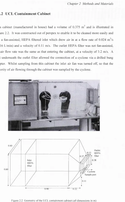
Figure 2.2 Geometry of the UCL containment cabinet... 45
Figure 2.3 The bead mill and its cabinet... 46
Figure 2.4 The Sharpies room ... 47
Figure 2.5 UCLa c b e fermentation h a ll... 48
Figure 2.6 UCLACBE downstream processing suite... 49
Figure 2.7 Glass atomiser... 51
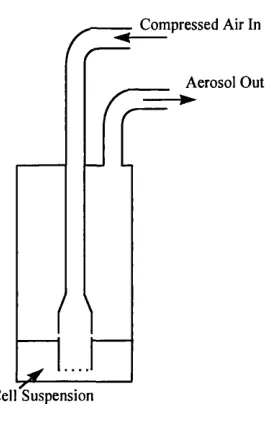
Figure 2.8 The Collison nebuliser... 52
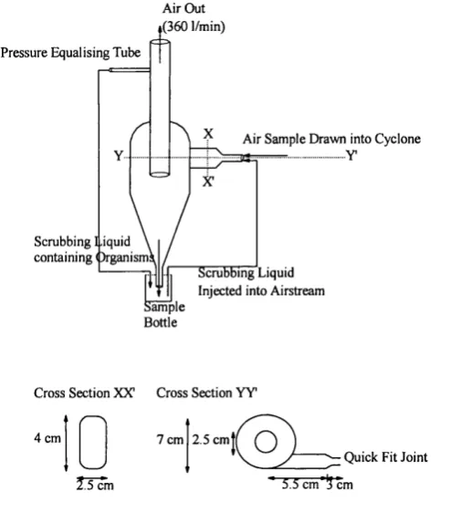
Figure 2.9 Schematic of cyclone operation... 53
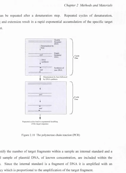
Figure 2.10 The polymerase chain reaction (PCR)...55
Figure 3.1 Disk space and CPU time required with respect to the number of control volumes used 58 Figure 3.2 Sequence of Operations for the SIMPLE and SIMPLEC Algorithms... 61
Figure 3.3 Control volume notation...67
Figure 3.4 Time dependence of velocity in a turbulent flow...71
Figure 3.5 Effect of the number of control volumes on the predicted air velocities in a 1.1 m^ containment cabinet... 76
Figure 3.6 The air flow patterns obtained in a l.lm^ cabinet when a different number of control volumes were used... 77
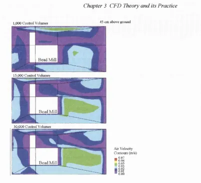
Figure 3.7 Effect of the number of control volumes on the predicted air velocities in a 45 m^ processing area... 78
Figure 3.8 Predicted and measured air velocity data at different positions in the Sharpies centrifuge room ... 78
Figure 3.9 Regions of grid refinement in the Sharpies centrifuge room ... 79
Figure 3.10 Comparison of the predicted air velocities using a refined and an unrefined g rid ...80
Figure 3.11 Converging iterative solution... 82
Figure 3.12 Steady-state solution of transient flow... 82
Figure 3.13 Diverging iterative solution... 83
Figure 3.14 Iterative solution with additional particle tracking loops...83
Figure 3.15 Air velocity vectors after 100 iterations... 84
Figure 3.16 Air velocity vectors after 500 iterations... 84
Figure 3.17 Residual plot at low under-relaxation factor...85
Figure 3.18 Residual plot at high under-relaxation factor... 86
Figure 3.19 Effect of the number o f control volumes on the predicted air velocities in the UCLACBE downstream processing suite... 87
Figure 3.20 Typical residual plot for Sharpies room simulations utilising a hybrid differencing scheme 88 Figure 3.21 Typical residual plot for Sharpies room simulations utilising a CCCT differencing scheme 88 Figure 3.22 Typical residual plot for downstream processing suite simulations utilising a hybrid differencing scheme... 89
Figure 3.23 Typical residual plot for downstream processing suite simulations utilising a CCCT differencing scheme... 89
Figure 3.24 Comparison of the measured and CFD air velocities when the hybrid and CCCT differencing schemes were used on a grid of 66,000 control volumes in the Sharpies room... 90
Figure 3.25 Comparison of the measured and CFD air velocities Im above ground, when the hybrid and CCCT differencing schemes were used on a grids of 96,000 and 121,000 control volumes in the downstream processing suite...92
Figure 3.26 Comparison of the measured and CFD air velocities 2m above ground, when the hybrid and CCCT differencing schemes were used on a grids of 96,000 and 121,000 control volumes in thedownstream processing suite...92
Figure 4.1 Variation of air velocity in the Bassaire cabinet with the number of control volumes u se d ... 99
defined as variable mass flow boundaries... 103
Figure 4.5 Predicted flow patterns and particle trajectories when the inlet was defined as a fixed flow boundary and the outlet as a variable flow boundary...103
Figure 4.6 Predicted flow patterns and particle trajectories when the inlet is defined as a variable flow boundary and the outlet as a fixed flow boundary... 104
Figure 4.7 Predicted particle trajectories in the simplified geometry, with the inlet and extraction fans turned off...;... 106
Figure 4.8 Predicted particle trajectories in the accurate geometry, with the inlet and extraction fans turned off... 106
Figure 4.9 Predicted particle trajectories in the simplified geometry, with the inlet and extraction fans turned on... 107
Figure 4.10 Predicted particle trajectories in the accurate geometry, with the inlet and extraction fans turned on... 107
Figure 4.11 Predicted particle trajectories in a larger cabinet (simplified geometry), with the inlet and extraction fans turned off...109
Figure 4.12 Predicted particle trajectories in a larger cabinet (accurate geometry), with the inlet and extraction fans turned off...109
Figure 4.13 Predicted particle trajectories in a larger cabinet (simplified geometry), with the inlet and extraction fans turned on...110
Figure 4.14 Predicted particle trajectories in a larger cabinet (accurate geometry), with the inlet and extraction fans turned on...110
Figure 4.15 Predicted particle trajectories of a release of E. coli... 113
Figure 4.16 Predicted particle trajectories of a release of S. cerevisiae...113
Figure 4.17 Predicted particle trajectories of a microbial release with a density of 1400 kg/m^ 114 Figure 4.18 Predicted particle trajectories of a microbial release with a density of 2300 k g W 115 Figure 4.19 Predicted particle trajectories of a microbial release with a density of 1400 kg/m^ and a coefficient of restitution of 0.2... 116
Figure 4.20 Predicted particle trajectories of a microbial release with a density of 2300 kg/m^ and a coefficient of restitution of 0.2... 116
Figure 4.21 Comparison of the spherical and non-spherical shapes used in the m odels... 117
Figure 4.22 Predicted particle trajectories of non-spherical organisms...118
Figure 4.23 Percentage of particles adhering to walls as a function of particle size... 121
Figure 5.1 Experimental collection efficiencies of micro-organisms in the Bassaire cabinet...123
Figure 5.2 Experimental collection efficiencies of micro-organisms in the UCL containment cabinet, when the organisms were released from different locations within the cabinet... 124
Figure 5.3 Variation of air velocities in the UCL containment cabinet with the number of control volumes used...127
Figure 5.4 Variation of air velocities in the UCLACBE fermentation hall with the number of control volumes used... 127
Figure 5.5 Typical residual plot for UCL containment cabinet simulations... 128
Figure 5.6 Typical residual plot for UCLacbe fermentation hall simulations...128
Figure 5.7 Predicted organism trajectories in the Bassaire cabinet when the organisms have a coefficient of restitution of 0.0 and a diameter of 1 fim...131
Figure 5.8 Predicted organism trajectories in the Bassaire cabinet when the organisms have a coefficient of restitution of 0.2 and a diameter of 1 pm ...131
Figure 5.9 Predicted organism trajectories in the Bassaire cabinet when the organisms have a coefficient of restitution of 0.0 and a diameter of 5 pm ...132
Figure 5.10 Predicted organism trajectories in the Bassaire cabinet when the organisms have a coefficient o f restitution of 0.2 and a diameter of 5 pm ...132
Figure 5.11 Predicted organism trajectories in the Bassaire cabinet when the organisms have a coefficient o f restitution of 0.0 and a diameter of 10 pm...133
Figure 5.14 Predicted trajectories of 5 pm organisms around the UCL containment cabinet...138 Figure 5.15 Predicted trajectories of 10 pm organisms around the UCL containment cabinet...138 Figure 5.16 Predicted percentage collection in cyclone as a function of the coefficient of restitution,
when microbial release occurred from position “Wall 1”...139 Figure 5.17 Predicted organism trajectories from position “Wall 1” in the UCL containment cabinet. The simulation assumed a particle size of 10 pm and a coefficient of restitution of 0.2... 139 Figure 5.18 Predicted organism trajectories from position “Wall 2” in the UCL containment cabinet The
simulation assumed a particle size of 10 pm and a coefficient of restitution of 0.2... 140 Figure 5.19 Comparison between experimental data and CFD predictions for the percentage of
organisms collected in the UCL containment cabinet, when released from different locations 141 Figure 5.20 Comparison between air velocities predicted by CFD and those measured by hot wire
anemometry in the UCLACBE fermentation hall...142 Figure 5.21 Percentage collection of zinc sulphate from different locations in the UCLa c b e fermentation
hall... 143 Figure 5.22 Predicted trajectory of released zinc sulphate in the UCLACBE fermentation hall, when the
coefficient of restitution was 0.0...144 Figure 5.23 Predicted trajectory of released zinc sulphate in the UCLACBE fermentation hall, when the
coefficient o f restitution was 0.2... 145 Figure 5.24 Comparison of the collection efficiency predicted by CFD and experimental collection of
zinc sulphate at different locations in the UC Lacbefermentation hall... 146
Figure 6.1 Cyclone attached to the side of the bead mill cabinet... 152 Figure 6.2 Simple diagram of bead mill components... 153 Figure 6.3 Predicted trajectory of a release of E. coli originating from the top of the Sharpies tubular
bowl centrifuge, when the coefficient of restitution is 0.0...155 Figure 6.4 Predicted trajectory of a release of E. coli originating from the top of the Sharpies tubular
bowl centrifuge, when the coefficient of restitution is 0.2...155 Figure 6.5 Predicted trajectory of a release of 1 pm organisms originating from the top of the Sharpies
tubular bowl centrifuge, when the coefficient of restitution is 0.2...156 Figure 6.6 Predicted trajectories of a release of E. coli, originating from the centrifuge bowl (end nearest
centrifuge), during transport of the bowl across the room. The organisms had a coefficient of restitution o f 0.0... 158 Figure 6.7 Predicted trajectories of a release of E. coli, originating from the centrifuge bowl (end nearest
centrifuge), during transport of the bowl across the room. The organisms had a coefficient of restitution o f 0.2... 158 Figure 6.8 Predicted trajectories of a release of E. coli, originating from the centrifuge bowl (end nearest
safety cabinet), during transport of the bowl across the room. The organisms had a coefficient of restitution o f 0.0... 159 Figure 6.9 Predicted trajectories of a release of E. coli, originating from the centrifuge bowl (end nearest
safety cabinet), during transport of the bowl across the room. The organisms had a coefficient of restitution o f 0.2... 159 Figure 6.10 Predicted trajectories of a release of E. coli originating from the centre of the bead mill
sieve. The organisms had a coefficient of restitution of 0.0... 161 Figure 6.11 Predicted trajectories of a release of E. coli originating from the centre o f the bead mill
sieve. The organisms had a coefficient of restitution of 0.2... 162 Figure 6.12 Predicted trajectories of a release of S. cerevisiae originating from the centre of the bead mill sieve. The organisms had a coefficient of restitution of 0.2... 164 Figure 6.13 Predicted trajectories of a release of E. coli, with a coefficient of restitution o f 0.2,
originating from the centre of the bead mill sieve. The cyclone was extracting air from a port on the opposite wall...165
Figure 7.3 Mechanisms for the movement of organisms around areas... 176
Figure 7.4 Air velocity contours in the UCLacbe downstream processing suite... 180
Figure 7.5. Predicted trajectories of a release of 5 pm organisms with a coefficient o f restitution of 0.2 in the UCLacbe downstream processing suite. Release occurs from the region of stagnant air 181 Figure 7.6. Predicted trajectories of a release of 5 pm organisms with a coefficient o f restitution o f 0.2 in the UCLacbe downstream processing suite. Release occurs from near the door... 181
Figure A 1 ADH process flowsheet... 196
Figure A2 a-amylase process flowsheet...196
Figure A3 Unit scores for the operations involved in the ADH process... 197
Figure A4 Hazard indices for different process routes in the a-amalylase process...198
Figure B1 Body-Fitted 2-Dimensional Grid Topologies...206
Figure C l Geometry of the Bassaire cabinet, showing dimensions, axes and the positions of the ports on the z=62 plane... 208
Figure C2 Geometry of the UCL containment cabinet, showing axes and dimensions along the z plane ... 209
Figure C3 Geometry of the UCL containment cabinet, showing axes and dimensions along the x=1.12 plane...209
Figure C4 Geometry of the beadmill cabinet, showing axes and dimensions along the y=0.9 plane.... 210
Figure C5 Geometry of the beadmill cabinet, showing axes and dimensions along the x=0 plane...210
Figure C6 Geometry of the beadmill... 211
Figure C7 Geometry of the Sharpies room, showing axes and dimensions along the y plane... 211
Figure C8 Geometry of the sharpies room, showing axes and dimensions along the z=3 plane...212
Figure C9 Geometry of the UCLACBE fermentation hall, showing axes and dimensions along the y plane...212
Figure CIO Geometry of the UCLACBE fermentation hall, along two planes on the x a x is...213
Figure Cl 1 Geometry of the UCLACBE fermentation hall, along the z=0 plane... 213
Figure C12 Geometry of the UCLACBE downstream processing suite, showing axes and dimensions along the y=3.25 plane... 214
Table 1.1 OECD Containment L evels...23
Table 1.2 Summary of UK Biosafety Legislation... 25
Table 1.3 Features of Clean Room s...31
Table 2.1 Micro-organisms Used in this Study...56
Table 3.1 Comparison of Finite Difference Schemes... 69
Table 3.2 The Advantages And Disadvantages of Different Turbulence Models... 75
Table 3.3 Turbulent Intensities in Processing Areas... 93
Table 3.4 Component Turbulent Intensities in Processing A reas... 94
Table 5.1 Variable Values Used in Bassaire Cabinet Simulations... 129
Table 6.1 Number of Organisms Enumerated by PCR for Each Sample... 150
Table 6.2 Number of Organisms Released from Centrifuge Bowl During it’s Transport Across the Room, Using a Combination of Quantitative PCR and CFD... 160
Table 7.1 Hardware and Software Costs for C F D ...172
Table 7.2 Destination of Organisms Following Release in the UCLACBE Downstream Processing Suite... 181 Table A1 Toxicity Scores... 193
Table A2 Organism Scores...193
Table A3 Pressure Scores... 195
Table A4 Temperature Scores...195
Table A5 Inventory Scores... 195
Table A6 Rotating Equipm ent...195
AAS Atomic Absorption Spectrophotometer ACDP Advisory Committee on Dangerous Pathogens ACGM Advisory Committee on Genetic Manipulation
ASM Algebraic Stress Model
CAD Computer Aided Design
CEI Chemical Exposure Index
CFD Computational Fluid Dynamics
CCCT Curvature Compensated Convection Transport COSHH Control o f Substances Hazardous to Health.
CPU Central Processing Unit
CV Control Volume
DNA Deoxyribose Nucleic Acid
EPA Environmental Protection Act
ETA Event Tree Analysis
F&EI Fire and Explosion Index
FMEA Failure Modes and Effects Analysis
FTA Fault Tree Analysis
GILSP Good Industrial Large Scale Practice HASAWA Health And Safety at Work Act. HAZOP Hazard and Operability Study HEPA High Efficiency Particulate Air
OECD Organisation for Economic Co-Operation and Development
PCR Polymerase Chain Reaction
Pe Peclet number
PISO Pressure Implicit with Splitting o f Operators
ppm Parts per million
QUICK Quadratic Upstream Interpolation for Convective Kinetics
RAM Random Access Memory
rDNA Recombinant Deoxyribose Nucleic Acid
RO Reverse Osmosis
RSM Reynolds Stress Model
SIMPLE Semi-Implicit Method for Pressure Linked Equations SIMPLEC Semi-Implicit Method for Pressure Linked
Equations-Consistent
SIMPLER Semi-Implicit Method for Pressure Linked Equations-Refined
TLV Threshold Limit Value
Symbols
A C E F k K m n N P P q s Se t T u V V w W X y zArea (m )
Computational position (-)
Node to the east o f the general node. (-) Force acting upon particle (N)
Turbulent kinetic energy (m^/s^) Thermal conductivity (W/m K) Mass (kg)
Number o f iterations (-)
Node to the north o f the general node (-) Pressure (N/m^)
General node (-) Heat flux (W/m^)
Node to the south o f the general node (-) Source term (-)
Time (s)
Temperature (K)
Velocity component in the Cartesian x-direction (m/s) Velocity component in the Cartesian y-direction (m/s) Volume (m^)
Velocity component in the Cartesian z-direction (m/s) Node to the west o f the general node (-)
Distance in the Cartesian x-direction (m) Distance in the Cartesian y-direction (m) Distance in the Cartesian z-direction (m)
Greek Symbols
a P r 8 Vt P e XUnder-relaxation factor (-) Curvature constant (-) Effective diffusivity (m^/s)
Rate o f dissipation o f turbulent kinetic energy (m^/s^) Eddy-viscosity (kg/m s)
Computational velocity (m/s) Density (kg/m^)
General property (-) Viscous stress (kg/m s^)
1.0 Introduction
1.1
Project Importance and Aims
1.1.1 The Need for a Quantitative Approach to Release from
Bioprocesses
The majority of large scale bioprocesses are recognised as being safe \ However,
some processes may involve a pathogenic organism or one which has been
genetically modified and, if hazardous to man or to the environment will, by law,
require containment
Current UK legislation in this area is qualitative in nature and states that microbial
release from a process must either be minimised or prevented, depending upon the
containment category under which the process is operating. The words “minimise”
and “prevent” are obviously subjective and difficult to interpret and to implement. It
would be better for both the regulatory authorities and the bioprocessing industry if
quantitative limits were set. However, there is little published data available at the
moment with regard to the release of micro-organisms from bioprocesses. Previous
studies which have monitored microbial release have tended to be of a qualitative
nature Thus, there is a need for a quantitative approach to the measurement of
releases from a bioprocess, both incidental during normal operation and accidental
due to mechanical failure or operator error.
1.1.2 Aims of the Project
The primary aim of this project was to relate what is captured in a sampling device to
the total release from a process. This thesis describes the use of Computational Fluid
Dynamics (CFD) to determine the effectiveness of sampling techniques and to assess
generating air flow data and a spatial particle distribution within a processing area,
then relating this to sampling information. In this way a quantitative assessment of
total microbial release may be determined, as can an indication of the best position to
place sampling devices.
1.2
UK Biosafety Legislation
This section will summarise the biosafety legislation as it now stands, it will explain
how this legislation came into being, highlight the problems associated with it and
explain why a more quantitative approach is required.
1.2.1 UK Legislation Concerning the Safe Use of Genetically
Modified Organisms
Firstly, the development of biosafety legislation will be explained followed by a
description of the current UK legislation. The section is summarised in Table 1.2.
1.2.1.1 Chronological Development of Biosafety Legislation
Th e Ro b e n s Re p o r t (1972) a n d t h e He a l t h a n d Sa f e t y a t Wo r k Ac t (1974)
All UK regulations concerning genetically modified organisms are made under the
power of the Health and Safety at Work Act ^ (1974), which makes general
provisions for the health and safety of individuals which apply to all workplaces.
The act came into existence as a direct result of recommendations made in the
Robens' Report ^ (1972). At the time the report was published there were no safety
regulations which encompassed all places of work. The report proposed unified
1. That a comprehensive act for health and safety at work should be passed, which
should be supported by a combination of regulations and non-statutory codes and
standards. The regulations should be limited to general requirements only,
detailed specifications on technical content should be undertaken by expert
technical working parties.
2. That what is now known as the Health and Safety Executive should be set up to
unify administrative arrangements and to provide a mechanism for linking
statutory activities in a more comprehensive way.
The Health and Safety at Work Act ^ (1974) places a general duty on the employer:
“...requiring the provision and maintenance o f a working environment fo r their
employees that is, so fa r as is reasonably practicable, safe without risks to health
and adequate as regards facilities and arrangements fo r their welfare at work. ”
The employer is also charged with the duty to avoid exposure of those not in his
employment, including the general public, to risks. The phrase “so far as is
reasonably practicable” qualifies these duties, such that the employer must carry out
a cost-risk analysis, balancing the risk involved in carrying out the work against the
cost of avoiding that risk.
The Go r d o n Research Conference on Nucleic Acids (1973)
The first attempt to regulate the use of recombinant DNA technology was made at
the Gordon Research Conference on Nucleic Acids held in the USA in 1973. The
conference gave a hearing to several papers which showed that DNA molecules from
separate sources could be covalently joined and transferred between living
organisms. It was recognised that this technique could pose unknown hazards and
committee on rDNA molecules and a voluntary embargo on certain DNA
manipulations was introduced. Two major problems were recognised:
1. The biological and ecological hazards of rDNA were not known.
2. Procedures to minimise the spread within humans and other populations had not
been developed.
T h e A s ilo m a r C o n f e r e n c e o n R e c o m b in a n t DNA M o l e c u l e s (1975)
The 1975 Asilomar Conference on Recombinant DNA Molecules recommended,
for the first time, that biological and physical barriers could be used to contain
recombinant micro-organisms. It recognised that the potential risks of rDNA
technology should be dealt with by incorporating containment as an essential feature
in experimental design and matching the level of containment used with the
estimated risk. It was suggested that experiments be classified into four different
categories: minimal, low, moderate and high, based on the risk involved. The
conference recommended the use of vectors and bacterial hosts with restricted
capacities to multiply outside of the laboratory and physical containment measures
such as the use of hoods, limited access, negative pressure and adherence to good
microbiological practices.
T h e O r g a n is a t io n f o r E c o n o m ic C o -O p e r a tio n a n d D e v e lo p m e n t (OECD)
G u id e lin e s (1986)
In the years following the Asilomer conference, the manufacture of proteins with
recombinant organisms grew in scale and it became necessary to control the larger-
scale processes. Much of the guidance on large-scale use is based on the
recommendations and conclusions of a major international study by the Organisation
for Economic Co-Operation and Development (OECD) This report gave
practices. It described the approach of Good Industrial Large Scale Practice (GILSP)
which is now in common practice throughout Europe and is the basis of the European
Directive on the Contained Use of genetically modified organisms (90/219/EEC)
(1990). The report described large scale (i.e., larger than 10 litres) containment
levels for genetically modified organisms ranging from GILSP through a series of
increasingly stringent levels of containment (categories 1 through to 3). The
differences between these categories are detailed in Table 1.1. The OECD
recognised that GILSP is not a containment category, but adopted it because many
organisms used in traditional manufacture are considered safe since they have been
used for many years and have not presented any problems. Similarly the report
stated that:
“In the same way, modified organisms prepared by inserting segments o f DNA that
are well characterised and free from known harmful sequences into such organisms
to improve their performance, are also unlikely to pose any risk. ”
The OECD guidelines are operational guidelines which attempt to control the scale
of release. Incidental release, however small, cannot be prevented so the guidelines
rely upon biological containment to kill genetically modified organisms once
released. The sets of large-scale guidelines from the US National Institutes of Health
and the Advisory Committee for Genetic Manipulation (ACGM) in the UK are
similar in outline to those from the OECD (1986). All are structured into a set of
three increasingly stringent levels of containment above a lower level comparable to
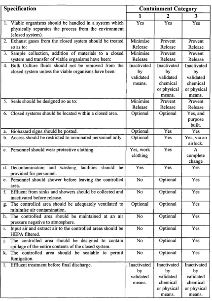
Table 1.1 OECD Containment Levels
Specification Containment Category
1 2 3
1. Viable organisms should be handled in a system which physically separates the process from the environment (closed system).
Yes Yes Yes
2. Exhaust gases from the closed system should be treated so as to:
Minimise Release Prevent Release Prevent Release 3. Sample collection, addition of materials to a closed
system and transfer of viable organisms have been:
Minimise Release Prevent Release Prevent Release 4. Bulk Culture fluids should not be removed from the
closed system unless the viable organisms have been:
Inactivated by validated means. Inactivated by validated chemical or physical means. Inactivated by validated chemical or physical means.
5. Seals should be designed so as to: Minimise
Release
Prevent Release
Prevent Release 6. Closed systems should be located within a closed area. Optional Optional Yes, and
purpose built.
a. Biohazard signs should be posted. Optional Yes Yes
b. Access should be restricted to nominated personnel only Optional Yes Yes, via an airlock.
c. Personnel should wear protective clothing. Yes, work
clothing
Yes A
complete change d. Decontamination and washing facilities should be
provided for personnel.
Yes Yes Yes
e. Personnel should shower before leaving the controlled area.
No Optional Yes
f. Effluent from sinks and showers should be collected and inactivated before release.
No Optional Yes
g. The controlled area should be adequately ventilated to minimise air contamination.
Optional Optional Yes
h. The controlled area should be maintained at an air pressure negative to atmosphere.
No Optional Yes
i. Input air and extract air to the controlled areas should be HEPA filtered.
No Optional Yes
j. The controlled area should be designed to contain spillage of the entire contents o f the closed system.
No Optional Yes
k. The controlled area should be sealable to permit fumigation.
No Optional Yes
1.2.1.2 Current UK Biosafety Legislation
Th e Co n t a i n e d Us e Re g u l a t i o n s (1992)
In 1992 the Genetically Modified Organism (Contained Use) Regulations ^ (1992)
were introduced, which replaced the earlier Genetic Manipulation Regulations
(1989). The regulations, which came into force in 1993, were made under the
powers of the Health and Safety at Work Act (1974) to cover human health and
environmental risks. “Contained Use” refers to any operation in which organisms
are genetically modified, or in which genetically modified organisms are cultured,
stored, used, transported, destroyed or disposed of.
The organism involved must be assigned to one of two hazard ranked groups. This
will be Group I for low or zero risk micro-organisms (equivalent to GILSP) and
Group II for micro-organisms which are hazardous to man or the environment. The
operation being carried out is assigned as Type A for research and teaching work or
Type B for commercial work. The level of containment must be determined, which
will be Bj (equivalent to GILSP), B2, B3, or B4 (equivalent to OECD large scale
categories 1, 2 and 3).
A risk assessment must then be performed which considers both human health and
the environment. This encompasses categorisation of the micro-organism and the
operation for notification and determination of appropriate control measures.
Table 1.2 Summary of UK Biosafety Legislation
Title Content
Health and Safety at Work Act (1974)"
• Made it the legal responsibility of employers to ensure the health, safety and Avelfare at work of all employees.
Organisation for Economic Co- Operation and Development
(OECD), rDNA Safety
Considerations (1986)
• Recommendations on the use of rDNA technology in agriculture, industry and the environment.
• A risk assessment was carried out on all organisms and processes were placed into physical containment categories. Containment of Substances
Hazardous to Health (COSHH) Regulations (HASAWA)
(1988)
• Protects employees from hazards, such as allergens, toxic products and carcinogens, connected with biological processes and products.
• Makes it the employer's duty to: assess health risks, control exposure and measure testing, do exposure testing and health surveillance and inform employees of risks in their work.
Advisory Committee on
Dangerous Pathogens (ACDP) (1989)
• Produced a guidance document on the classification of pathogens according to the inherent hazard of the organism.
Advisory Committee on Genetic Manipulation (ACGM) (1987)
• Guidance notes to support Genetic Manipulation Regulations (1989)
• Requires the formation of a Genetic Manipulation Safety Committee at a local level, to assist in the assessment of risks from proposed work and to decide on a containment level.
• Note 6 relates to the large scale use of genetically modified organisms. Note 7 relates to the risk assessment of operations involving the use of such.
Environmental Protection Act (EPA) (1990)
• Intended to regulate on internationally agreed principles, put the safety of people and the environment first and where possible allow relaxation of control measures where indicated by experience.
Genetically Manipulated
Organism (Deliberate Release) Regulations (1992)
• Introduced in compliance with EC Directive 90/220/EEC (under the EPA) to deal with the deliberate release of Genetically Manipulated Organisms into the environment. Genetically Modified Organism
(Contained Use) Regulations (1992)^
(Replaced Genetic Manipulation Regulations (1989) ^®)
• Introduced in compliance with EC Directive 90/219/EEC (under the HASAWA) to deal with the use of genetically modified organisms in teaching, research and industry.
• Introduced nomenclature for organism, process and containment level.
• Requires risk assessment to consider risks to human health and environment.
1.2.2 The Practical Implications of Current Legislation
Current legislation is qualitative in nature and is thus subjective and difficult to
interpret and implement. Terms such as “m inim ise release” and “prevent release” are
inadequately defined and are difficult to translate into m echanical engineering design
adhered to and this has led to some confusion over the interpretation of the
legislation. Industry has reacted to biosafety legislation by applying more
containment measures than are necessary, which inevitably leads to higher plant
costs and processes which are more difficult to work with. The arguments over
the appropriate seal design for different containment levels illustrates the problem.
The following seal specifications have been proposed at different containment
23
categories :
• Single static seal for OECD large scale containment category 1 (see section
1.2 .1.1).
• Double static seal for OECD large scale containment category 2 (section 1.2.1.1).
• Double static seal with barrier fluid/steam trace for OECD large scale containment
category 3 (section 1.2.1.1).
However, this interpretation of the legislation has been criticised as a simplistic
model lacking any real validation. It has been pointed out that the assumption that
two static seals are better than one is not necessarily valid Double static seals can
be criticised on several counts: they are more difficult to assemble correctly and so
risk of failure may be increased; it is difficult to detect failure of either seal in
operation. Both seals will have similar histories, therefore the possibility of
simultaneous failure might be higher than anticipated. The interpretation of the
regulations described above may therefore lead to the adoption of inappropriate, and
possibly costly, engineering features. A report in 1993 by the Select Committee on
Science and Technology expressed concern that the current biosafety regulations
would lead to a lack of competitiveness in the UK biotechnology industry.
The difficulties experienced by industry as the use of genetically modified organisms
has become more widespread across a large number of sectors, has been attributed to
the following
2. The attempt to apply the same containment parameters to all sectors, when these
particular parameters are more applicable to only a small area of the total
biotechnology industry.
3. The administrative burden placed on industry by existing legislation.
A quantitative approach to the release of micro-organisms from large scale processes
is important, in order that the regulatory authorities can categorise containment levels
in a more precise manner. Less subjective legislation would be easier to apply
universally and would reduce the confusion which currently exists across industry.
1.3
Biosafety Aspects of Facility Design and Downstream
Processing Unit Operations.
Having discussed biosafety legislation and the levels of containment required, this
section will describe the types of containment which are possible and the design
considerations which are necessary for a contained facility. It then considers the
biosafety aspects of some of the typical unit operations encountered in bioprocessing.
1.3.1 Bioprocess Facility Design for Biosafety
Bioprocesses have been defined as open or closed systems An open system is one
in which material enters the process from or exits to the external environment. The
material could be solvent vapour emerging from the top of a vessel or an aerosol
release from a unit operation. A closed system is one in which no material passes to
or from the external environment.
A closed system, since it does not allow any material to escape from the process-
including leakage of vapour aerosol or dust from unit operations, is defined as
achieve. Primary containment has been defined as “...the protection o f personnel
and the immediate vicinity o f the process from exposure to process materials (which
is) provided by appropriate equipment and the use o f safe operating procedures. ”
The equipment required for primary containment is mechanically complex, must be
operated correctly and kept in good repair Its design should incorporate the
following
• All equipment containing live organisms should be steam sterilisable and have a
sterile vent filter.
• Exhaust gases from contained vessels should be filtered.
• Special consideration should be given to seals on flange joints, instrument probes,
etc. This may involve single or double O rings and possibly steam sterilisation.
• Rotating shafts, such as agitators, may require a double-acting mechanical seal
with a steam or condensate trace.
• Operation of a steam barrier between contained vessels.
• Sterilisation prior to discharge of waste streams.
An open system can achieve secondary containment, in which the facility becomes
part of the process. A secondary containment barrier has been described as a
physical and operational barrier erected around the process to isolate it from the
external environment Secondary containment has been defined as “...the
protection o f personnel and the environment external to the facility from exposure to
process materials (which is) provided by a combination o f facility design and
operating practices. ” The following concepts would be incorporated into the
design of a secondary containment facility
• The contained area should be physically separated from other building functions,
usually by an ante room.
• The contained area should be able to contain accidental spillage’s. This may be
achieved by having the floor recessed slightly below adjacent areas and sloping
towards drains.
• OECD large scale containment category 3 (section 1.2.1.1) areas must be
completely sealable to enable the area to be fumigated.
In order to isolate the secondary containment area from the outside environment air
will be HEP A filtered (see section 1.3.1.1) and perhaps a pressure differential will
exist between the contained area and it's surrounding (see section 1.3.1.2).
1.3.1.1 High Efficiency Particulate Air (HEPA) Filters
In a contained facility the exhaust air will be passed through a high efficiency
particulate air (HEPA) filter. In some cases incoming air is also filtered to reduce the
microbial burden in the room. A HEP A filter is rated by its efficiency in removing
particles greater than 0.3 pm and typically have a rating of 99.97 %. Under ideal
conditions HEP A filters have been shown to be 99.9999 % efficient in collecting
bacterial spores and 99.999 % efficient in collecting viruses thus providing an
effective barrier between the process and the external environment.
The efficiency of a HEP A filter is affected by the air velocity across it and also by
the amount of filtering medium it contains Traditional HEP A filters consist of
rolls o f filter paper folded back and forward, the folds of paper being separated by a
crinkled sheet of foil which gives the filter strength and allows air to pass through it.
Modem filters do not use a separator, the filter paper is merely folded allowing a
more compact filter to be constmcted.
The filter medium is generally made of synthetic fibrous materials and particulate
matter is separated from the bulk flow by impacting upon these fibres or upon
previously captured particles. Once attached the particulate matter will not be re
entrained. There are several capture mechanisms. As air flows around a fibre, larger
particles with sufficient momentum will leave the air stream and impact upon a fibre.
particles. This random motion causes them to come into contact with the fibres
where they are retained. Other particles are captured as they pass a fibre tangentially.
1.3.1.2 Negative Pressure Control
For OECD large scale containment category 3 (section 1.2.1.1) there is a requirement
that a contained area is maintained at negative pressure relative to its surroundings.
Negative pressure is obtained by extracting more air from the room than is supplied.
Often a negative pressure room will be entered via an ante room which provides an
additional barrier to the organisms and limits the impact of opening and closing
doors. It has been suggested that the exact pressure differential between the
contained area and its surroundings should be 15 Pa^^, however there do not appear
to be any hard and fast rules.
1.3.1.3 Clean Room Design
Since secondary containment facilities have similar fundamental design principles to
clean rooms, the next section considers the history of and principles behind clean
room design. Clean rooms originated from the need to control infection in hospitals.
In recent years a clean environment has become necessary for the industrial
manufacture of a diverse range of products. In the micro-electronics industry a clean
area is required to prevent submicron sized impurities from contaminating the
product, whilst the pharmaceutical/medical sector needs to prevent micro-organisms
from infecting a product or patient.
Clean rooms are classified into two types, depending upon their method of
ventilation. In a conventional, or turbulently-ventilated, room cleanliness is
dependent upon the quantity and quality of the air supplied and the efficiency with
which it mixes. In a uni-directional, or laminar, room the air flow is in one direction
removes contaminants by dilution and mixing, in a uni-directional room the air
velocity is high enough to remove all particles before they settle onto surfaces. The
cleanliness o f a room is also dependent upon the production o f contamination within
the room, which can be caused by people or machinery.
It has been known since the 1860’s that directional airflow was required for the
efficient removal of airborne contaminants Details of a clean area were reported
in 1946, which was pressurised with respect to the surrounding area and had 20 air
changes per hour of filtered air Early work also revealed the effectiveness of the
34,35
downward displacement of air
A summary of the key features of clean rooms is given in Table 1.3.
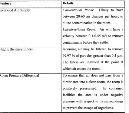
Table 1.3 Features of Clean Rooms
Feature: Details:
Increased Air Supply Conventional Room: Likely to have
between 20-60 air changes per hour, to
dilute contamination in the room.
Uni-directional Room: Air will have a
velocity between 0.3-0.45 m/s to remove
contaminants before they settle.
High Efficiency Filters Incoming air may be filtered to remove
99.97 % of particles greater than 0.3 pm.
The filters are installed at the point at
which air enters the room.
Room Pressure Differential To ensure that air does not pass from a
dirtier area into a clean room, the room is
positively pressurised. In contained
facilities the area is under negative
pressure with respect to its surroundings
1.3.2 Bioprocessing Unit Operations
The next section will look at the different operations used in the downstream
processing of a product. In particular, it will examine the hazard posed by each piece
of equipment with regard to the release of micro-organisms.
The most hazardous operations in terms of worker and environmental exposure are
material transfers, extraction and concentration ^6, The potential exposure hazard
increases as the product concentration increases at each production stage. In the
chemical industry the probability of a pipeline breakage, for a pipe in the open air,
has been calculated to be 10'^ per year In bioprocessing, fluids tend to be more
aqueous, substances are less aggressive and operating temperatures and pressures
tend to be lower, thus the probability of failure would be expected to be lower.
Therefore, breakage is less important than leakage. However, this may not be true in
a pilot plant facility which by its very nature uses interchangeable equipment and
connections. In this case inadequate setting up of the machinery may cause
accidents, particularly as the process becomes more complex.
When a force is exerted on a liquid a small aerosol droplet is formed which may have
a diameter small enough to access all parts of the respiratory tract. Aerosols can be
generated from any liquids involved in fermenter inoculation procedures, sampling,
vessel over pressure situations and drug recovery operations. Centrifuges and
homogenisers have the potential to produce aerosols of allergenic biological material.
Accidental spills often occur due to leaks in fermentation equipment, during the
transfer of process fluids and in recovery operations such as filtration.
A lot of attention has focused on incidental release of micro-organisms in aerosols,
since in such a state the released organisms may pose a threat to health and the
environment and can not be easily contained In addition, bioaerosols are
implicated in the transmission of disease in a variety of different situations ranging
from sewage worker exposure to “sick building syndrome” Any process such as
breaks down into small droplets and evaporates to form an aerosol. The amount of
aerosol produced from a liquid leak depends upon the cell concentration in the liquid,
the size of the opening, the velocity of the escaping fluid and the obstacles
encountered by the fluid. If the escaping fluid hits the surface of other apparatus,
-6
secondary aerosols may be produced. Aerosols are reported to contain 10 times the
total number of bacteria escaping in a fluid and in one inhalation a person will inhale
500-600 cells
The ability of any particular aerosol to cause infection or escape containment will
depend upon a range of characteristics of that aerosol. The properties of aerosols that
are important in terms of biosafety are the concentration of hazardous material and
the particle size distribution. In terms of micro-organisms, their concentration in the
process liquid will be greatest towards the end of the fermentation and in the early
stages of downstream processing, this will be reflected in the composition of any
aerosols produced.
The particle size distribution in an aerosol is dependant on the manner in which the
aerosol was produced and the nature of the liquid from which it is derived. The size
of particles in an aerosol is critical in determining the length of time a particle will
remain airborne. The larger aerosol droplets (>5 pm) sediment rapidly and the
organisms they contain may contaminate the bench and the operator's hands. Smaller
droplets dry rapidly in the air and leave the microbial particles suspended. If
particles of less than 5 pm diameter are inhaled, they may reach the alveoli and cause
infection while larger droplets are filtered and removed in the upper respiratory
tract
As well as the properties of the aerosol itself, external factors, such as the
surrounding air movement, temperature and humidity, will effect the dispersal of
micro-organisms. The interaction between these will determine the fate of an
aerosolised microbial release in the environment. Computational Fluid Dynamics
can be used to investigate the effect of these factors upon the movement of micro
1.3.2.1 Centrifugation
Centrifugal sedimentation is the principal method used for the harvesting of
fermentation broths and the recovery of biological products. The main advantages of
centrifugation include
1. Short retention times.
2. Small space requirements.
3. Adjustable separation efficiency for a particular product.
4. Closed systems. All running parts are enclosed and functional parts are controlled
hydraulically or pneumatically.
The safe operation of centrifuges can present problems, particularly because many
processes involve the fractionation of proteins from fermentation broths so a higher
level of biologically toxic materials persists through several processing stages.
Rotating machinery can disperse these substances in aerosol form, which presents a
hazard. For batch machines a biosafety problem may be created by the handling of
solids by the process operators.
A high speed disc stack centrifuge was monitored following the deliberate leakage of
10 mL of supernatant at low pressure ^ where the release was of a mutant strain of E.
coll. The centrifuge was placed inside a soft-film cabinet to provide secondary
containment and also to allow the air around the cabinet to be monitored. Inlet air
was HEP A (High Efficiency Particulate Air Filter) filtered and had a high enough
flow rate to provide a positive pressure inside the cabinet. Settle plates, both close to
the leak and further away, revealed that viable cells were present, therefore the
release must have been at least partly aerosolised. The acceptability of such an
accidental release during operation would depend upon the organism involved and its
effect on personnel and the environment.
Several incidents have been reported where the use of centrifuges has caused health
centrifuge led to the generation of an aerosol of Brucella abortus which was
disseminated throughout a building, infecting 45 people, one fatally Severe
allergic effects in four workers were reported in a French pharmaceutical company,
caused by the generation of a tuberculin aerosol by a centrifuge In the 1960's five
workers at University College London were affected by Pseudomonas aeruginosa
cell debris during a tubular bowl centrifugation operation In this last example,
modification of the type of centrifuge used has been successful in preventing any
recurrence of this type of incident.
1.3.2.2 Microfiltration
Microfiltration can be used for cell and cell debris removal, enabling product
recovery from the permeate or the concentration of a cell suspension prior to
disruption. It has an advantage over centrifugation in that, other than ancillary
equipment such as pumps, it does not include any high speed rotating parts, thus
aerosol formation is less likely. The main advantages of microfiltration include 42;
1. Operation at ambient temperature.
2. High separation efficiency.
3. Performance independent of cell size or density.
4. Good containment.
5. Compact, simple and reliable equipment.
1.3.2.3 Homogenisation
Cell disruption constitutes the first stage in the isolation of intracellular enzymes. It
entails breaking open the cell structure to release the intracellular product for its
subsequent recovery. A high disruption yield at this step will allow more flexibility
in the subsequent processing of the product The complete recovery of