computation
Article
Computation and Experiment on Linearly and
Circularly Polarized Electromagnetic Wave
Backscattering by Corner Reflectors in an
Anechoic Chamber
Mohammad Nasucha1,2,*, Josaphat T. Sri Sumantyo1, Cahya E. Santosa1, Peberlin Sitompul1, Agus H. Wahyudi1, Yang Yu1and Joko Widodo1
1 Center for Environmental Remote Sensing, Graduate School of Science and Engineering, Chiba University, Chiba 263-8522, Japan; [email protected] (J.T.S.S.); [email protected] (C.E.S.);
[email protected] (P.S.); [email protected] (A.H.W.); [email protected] (Y.Y.); [email protected] (J.W.)
2 Department of Informatics, Universitas Pembangunan Jaya, Tangerang Selatan 15413, Indonesia
* Correspondence: [email protected]; Tel.:+81-070-4404-4451
Received: 22 August 2019; Accepted: 21 September 2019; Published: 24 September 2019
Abstract:Electromagnetic wave backscattering by corner reflectors in an anechoic chamber is studied using our developed computational tool. The tool applies the Finite-Difference Time-Domain (FDTD) method to simulate the propagation of the wave’s electric and magnetic fields. Experimental measurement in an anechoic chamber is also carried out as a comparison. The two results show agreement, including the finding that the backscatter intensity variation amongst the four circularly polarized modes is significantly smaller than the variation amongst the four linearly polarization modes.
Keywords: computation in radar; computation in synthetic aperture radar; backscattering by corner reflectors; simulation on circularly polarized electromagnetic waves
1. Introduction
Understanding electromagnetic (EM) wave backscattering by corner reflectors is of interest to radar researchers. In particular, the backscattering of circularly polarized (CP) EM waves is of great interest. To study these CP EM waves, computations can be useful.
The articles [1–9] report previously done computations on EM wave distribution in an anechoic chamber, but not in the context of backscattering by corner reflectors or in the context of CP EM waves. These works contributed to the development and performance improvement of the anechoic chamber. The articles [10–16] report computations and analyses on EM wave backscattering by corner reflectors. However, most of the reported computations for EM waves were done for non-polarized and linearly polarized waves. Until today, only [10] reports a computation on circularly polarized EM waves. It used the Method of Moments, and the report did not present any technical details about how the circular polarization was realized.
To respond to this situation, our research aims to study circularly polarized EM wave backscattering by corner reflectors in an anechoic chamber through a computation using the Finite-Difference Time-Domain (FDTD) method. There has been no such work reported thus far. As an addition, we did the same computation for linearly polarized (LP) EM waves. An equivalent experiment has also been carried out to obtain a comparison.
Computation2019,7, 55 2 of 17
The simulation was done using our developed computational tool, called Anechoic Chamber Simulation Tool Version 1 (AST_V1). Both the simulation and the experiment were done for four target types, i.e., triangular trihedral, horizontal plate bar, vertical plate bar, and sphere, and for all linear polarization and all circular polarization modes.
The remainder of this article is arranged as follows: Section2addresses the method, Section3 reports the results, Section4discusses the results, and Section5summarizes the content of all sections.
2. Method
2.1. The Measurement Plan
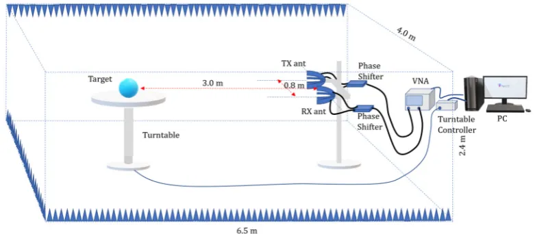
The measurement plan is depicted in Figure1. This was the scenario to be followed by both the computation and the experiment. It can be described as follows:
i. The cuboid anechoic chamber size shall be 6.5 (length)×4.0 (width)×2.4 m (height). ii. The distance between the transmitter (TX) and the receiver (RX) antennas shall be 0.8 m. iii. The distance between the target (corner reflector) and antennas in the orthogonal direction
shall be 3.0 m.
iv. The vector network analyzer (VNA)’s port 1 shall feed signals to the TX antenna. v. The RX antenna shall feed signals to the VNA’s port 2.
vi. The turntable shall be controlled by the turntable controller.
vii. Both the VNA and the turntable controller can be driven by the Personal Computer (PC). viii. Phase shifters shall be provided for the TX and RX antennas in the case of circular polarization
and shall be installed correctly for each mode, i.e., RX right-handed TX right-handed (RR), RX left-handed TX right-handed (LR), RX left-handed TX right-handed (LR), or RX left-handed TX left-handed (LL). Phase shifters will not be needed for linear polarization modes, i.e., RX horizontal TX horizontal (HH), RX vertical TX horizontal (VH), RX horizontal TX vertical (HV), and RX vertical TX vertical (VV).
ix. The transmit power shall be 5 dBm for all measurement cases.
x. The target shall be placed on a turntable in such a way so that elevation angleθ=0◦, and be rotated in such a way so that the aspect angleφchanges from−90◦to 90◦(negative and positive signs respectively represent the left and the right sides of the target) with 5◦increments. xi. The EM wave frequency shall be chosen in such a way so that 5λ<target size<10λ.
Computation 2019, 7, x FOR PEER REVIEW 2 of 16
The simulation was done using our developed computational tool, called Anechoic Chamber Simulation Tool Version 1 (AST_V1). Both the simulation and the experiment were done for four target types, i.e., triangular trihedral, horizontal plate bar, vertical plate bar, and sphere, and for all linear polarization and all circular polarization modes.
The remainder of this article is arranged as follows: Section 2 addresses the method, Section 3 reports the results, Section 4 discusses the results, and Section 5 summarizes the content of all sections.
2. Method
2.1. The Measurement Plan
The measurement plan is depicted in Figure 1. This was the scenario to be followed by both the computation and the experiment. It can be described as follows:
i. The cuboid anechoic chamber size shall be 6.5 (length) × 4.0 (width) × 2.4 m (height). ii. The distance between the transmitter (TX) and the receiver (RX) antennas shall be 0.8 m. iii. The distance between the target (corner reflector) and antennas in the orthogonal direction shall
be 3.0 m.
iv. The vector network analyzer (VNA)’s port 1 shall feed signals to the TX antenna. v. The RX antenna shall feed signals to the VNA’s port 2.
vi. The turntable shall be controlled by the turntable controller.
vii. Both the VNA and the turntable controller can be driven by the Personal Computer (PC). viii. Phase shifters shall be provided for the TX and RX antennas in the case of circular polarization
and shall be installed correctly for each mode, i.e., RX right-handed TX right-handed (RR), RX left-handed TX right-handed (LR), RX left-handed TX right-handed (LR), or RX left-handed TX left-handed (LL). Phase shifters will not be needed for linear polarization modes, i.e., RX horizontal TX horizontal (HH), RX vertical TX horizontal (VH), RX horizontal TX vertical (HV), and RX vertical TX vertical (VV).
ix. The transmit power shall be 5 dBm for all measurement cases.
x. The target shall be placed on a turntable in such a way so that elevation angle θ= 0°, and be rotated in such a way so that the aspect angle ϕchanges from –90° to 90° (negative and positive signs respectively represent the left and the right sides of the target) with 5° increments. xi. The EM wave frequency shall be chosen in such a way so that 5λ < target size < 10λ.
Figure 1. The measurement plan. The pyramidal absorbers shall be placed evenly at the inner sides of all six chamber’s walls.
Definitions of the elevation angle θ and the aspect angle ϕ are explained in Figure 2. The targets were corner reflectors of four different shapes: Trihedral, horizontal bar, vertical bar, and sphere. To make it realistic for practices, every target was chosen to be large enough compared to the wavelength
Computation2019,7, 55 3 of 17
Definitions of the elevation angleθand the aspect angleφare explained in Figure2. The targets were corner reflectors of four different shapes: Trihedral, horizontal bar, vertical bar, and sphere. To make it realistic for practices, every target was chosen to be large enough compared to the wavelength but not too large to be carried in a radar mission. Here we use the term “medium size” to specify that 5λ<target size<10λ. The targets and their descriptions are listed in Table1. The horizontal and the vertical plate bars are simply the same object, only having different standing orientations.
Computation 2019, 7, x FOR PEER REVIEW 3 of 16
but not too large to be carried in a radar mission. Here we use the term “medium size” to specify that 5λ < target size < 10λ. The targets and their descriptions are listed in Table 1. The horizontal and the vertical plate bars are simply the same object, only having different standing orientations.
Figure 2. Definitions of angles used in this work. The elevation angle θis the angle between the target’s facing direction and the horizontal plane. The aspect angle ϕ is the electromagnetic (EM) wave incident angle in the azimuth point of view (in other words, the angle between the target’s facing direction and the vertical plane). Every measurement case in this study shall be done with θ= 0° and –90° ≤ϕ≤ 90°.
Table 1. List of targets and their descriptions.
No. Target Description
1 Sphere A conducting thin-plate sphere having a diameter of 26 cm 2 Trihedral A conducting thin-plate triangular trihedral having a width of 64 cm 3 Horizontal bar A conducting thin-plate bar of 4 × 63 cm
4 Vertical bar The same as target no. 3 but vertically positioned
2.2. The Method of Computation
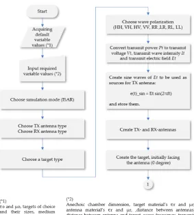
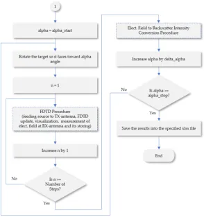
The computation was done systematically to fulfill the measurement plan specified in Section 2.1. A project definition, software requirement review, preliminary design review, and critical design review were carried out before coding and implementation [17]. The critical design review (CDR) of the AST_V1 is presented in Figures 3 and 4. The tool requires default input data, including the permittivity and the permeability of free space, and the relative permittivity (dielectric constant) and the relative permeability of the air (because the transmission medium in the experiments is the air). However, these values can be approximated by 1. The tool needs simulation case-related data, including the anechoic chamber size; the type, size, and material properties of corner reflector; the type and the material properties of the antennas; the distance between the TX and RX antennas; the distance between the antennas and the corner reflector; the polarization mode (either HH, VH, HV, VV, RR, LR, RL, or LL); and the Nyquist factor. The larger the Nyquist factor chosen by the user, the smaller the FDTD cell size configured by the tool will be, and thus the more accurate the simulation results can be expected to be while more computer resources will be consumed.
The field distribution was simulated using the FDTD method by applying the Yee-grid configuration [18,19], employing an electric- and magnetic-fields update technique based on Maxwell equations [18–22], and realizing the energy-absorbing walls of the anechoic chamber with perfectly matched layers (PMLs) [20].The real size of the anechoic chamber is 6.5 (length) × 4.0 (width) × 2.4 m (height). However, to minimize the usage of computer resources, the computation space domain was reduced to 4.2 (length) × 2.2 (width) × 2.0 m (height). The cuboid space domain was chosen in such a way that it is small enough but still contains all the objects of interest, i.e., the TX antenna, the RX antenna, and the corner reflector. This arrangement is valid because EM wave paths between the TX antenna and the corner reflector, and between the corner reflector and the RX antenna are “line of sight”. This computation space domain was realized by a Yee-grid consisting of 337 × 177 × 161 (9.6
Figure 2.Definitions of angles used in this work. The elevation angleθis the angle between the target’s facing direction and the horizontal plane. The aspect angleφis the electromagnetic (EM) wave incident angle in the azimuth point of view (in other words, the angle between the target’s facing direction and the vertical plane). Every measurement case in this study shall be done withθ=0◦and –90◦≤φ≤90◦.
Table 1.List of targets and their descriptions.
No. Target Description
1 Sphere A conducting thin-plate sphere having a diameter of 26 cm 2 Trihedral A conducting thin-plate triangular trihedral having a width of 64 cm 3 Horizontal bar A conducting thin-plate bar of 4×63 cm
4 Vertical bar The same as target no. 3 but vertically positioned
2.2. The Method of Computation
Computation2019,7, 55 4 of 17
Computation 2019, 7, x FOR PEER REVIEW 4 of 16
million) cells, where the cell size was 1.25 × 1.25 × 1.25 cm. With a lambda of 10 cm (f = 3 GHz), this cell size corresponds to a Nyquist rate of 8, which is well above the minimum Nyquist rate, i.e., 2.
Figure 3. Critical design review of Anechoic Chamber Simulation Tool Version 1 (AST_V1) presented in a flow chart (part 1).
Figure 3.Critical design review of Anechoic Chamber Simulation Tool Version 1 (AST_V1) presented in a flow chart (part 1).
Computation2019,7, 55 5 of 17
Computation 2019, 7, x FOR PEER REVIEW 5 of 16
Figure 4. Critical design review of AST_V1 presented in a flow chart (part 2).
In the computation, before the FDTD iteration, several procedures were carried out. The TX and RX antennas were synthesized, and targets were also synthesized and rotated according to the requested aspect angle ϕ. The transmitted power was converted to the transmitted voltage, transmitted wave intensity, and transmitted electric field. The transmitted electric field was represented in sinusoidal waves and fed carefully to the TX antenna by considering the requested mode of polarization.
For each mode of linear polarization, i.e., RX Horizontal–TX Horizontal (HH), RX Vertical–TX Horizontal (VH), RX Horizontal–TX Vertical (HV), or RX Vertical–TX Vertical (VV), either the TX horizontal or TX vertical antenna was fed with the sinusoidal waves. For each mode of circular polarization, i.e., RR, LR, RL, or LL, more attention was required since both the TX horizontal and TX vertical antenna needed to be fed simultaneously with the same train of sinusoidal waves, but of different phases.
During the iteration of the FDTD calculation, the value of the electric field arriving at the RX antenna was stored at every step. Upon completion of the calculation iteration, the set of stored electric field values was converted to the received wave intensity and optionally received power. The backscattered wave intensity in dB was calculated by:
BS Intensity (dB) = 10 log( ) (1)
where It is the intensity of the transmitted wave and Ir is the intensity of the received wave. Since the intensity equals the voltage amplitude squared, while the voltage is proportional to the electric field, the backscattered wave intensity can be alternatively obtained by:
BS Intensity (dB) = 20 log( ) (2)
where Et is the electric field transmitted by the TX antenna and Eris the electric field received by the RX antenna.
Figure 4.Critical design review of AST_V1 presented in a flow chart (part 2).
For each mode of linear polarization, i.e., RX Horizontal–TX Horizontal (HH), RX Vertical–TX Horizontal (VH), RX Horizontal–TX Vertical (HV), or RX Vertical–TX Vertical (VV), either the TX horizontal or TX vertical antenna was fed with the sinusoidal waves. For each mode of circular polarization, i.e., RR, LR, RL, or LL, more attention was required since both the TX horizontal and TX vertical antenna needed to be fed simultaneously with the same train of sinusoidal waves, but of different phases.
During the iteration of the FDTD calculation, the value of the electric field arriving at the RX antenna was stored at every step. Upon completion of the calculation iteration, the set of stored electric field values was converted to the received wave intensity and optionally received power. The backscattered wave intensity in dB was calculated by:
BS Intensity(dB) = 10 log(Ir It
) (1)
whereItis the intensity of the transmitted wave andIris the intensity of the received wave. Since the intensity equals the voltage amplitude squared, while the voltage is proportional to the electric field, the backscattered wave intensity can be alternatively obtained by:
BS Intensity(dB) = 20 log(Er Et
) (2)
whereEtis the electric field transmitted by the TX antenna andEris the electric field received by the RX antenna.
Computation2019,7, 55 6 of 17
circle rotation turntable for the device under test (DUT), which has two horizontal dipole antennas and two vertical dipole antennas.
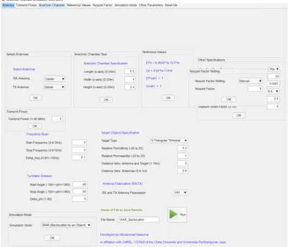
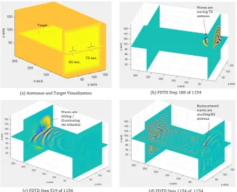
The AST_V1 user interface’s appearance is shown in Figure5. The four target types synthesized by the tool are shown in Figure6. Some visualization frames during a simulation are presented in Figure7, where target type=trihedral,f =3 GHz, polarization mode=RR,θ=0◦, andφ=0◦. In this figure, the target structure, the antenna structure, and the electric field distribution within the cuboid 3D space are visualized by applying one horizontal cutting plane and one or two vertical cutting plane(s).
It is necessary to mention that every cuboid shown in the figures visualizes a 3D space that is smaller than the anechoic chamber, because it represents only the FDTD space domain. This space domain reduction technique is applied to reduce computation time. The computation was done with a personal computer that uses an Intel CORE i7 processor and a set of 32 GB random access memory (RAM).
For future operations, in addition to the usage of dipole antennas, the tool can be equipped with more antenna choices, e.g., the circularly polarized microstrip antenna [23] that can handle a frequency range of 4.83 to 5.71 GHz. If the tool is modified to handle lower-frequency operations, it can be equipped with lower-frequency antennas, e.g., the circularly polarized microstrip antenna [24] that can handle frequencies of around 2.2 GHz. If it is intended to do simulations for higher frequencies, it can be equipped with, for example, the circularly polarized microstrip [25] that can operate in frequencies of around 9.4 GHz.
Computation 2019, 7, x FOR PEER REVIEW 6 of 16
The software has now become a graphical user interface (GUI) tool, namely AST_V1. The tool is currently capable of handling simulations on EM wave backscattering in an anechoic chamber with a size range of between 2 × 2 × 2 m to 20 × 20 × 20m in the frequency range of 3 to 8 GHz, with a full circle rotation turntable for the device under test (DUT), which has two horizontal dipole antennas and two vertical dipole antennas.
The AST_V1 user interface’s appearance is shown in Figure 5. The four target types synthesized by the tool are shown in Figure 6. Some visualization frames during a simulation are presented in Figure 7, where target type = trihedral, f = 3 GHz, polarization mode = RR, θ= 0°, and ϕ= 0°. In this figure, the target structure, the antenna structure, and the electric field distribution within the cuboid 3D space are visualized by applying one horizontal cutting plane and one or two vertical cutting plane(s).
It is necessary to mention that every cuboid shown in the figures visualizes a 3D space that is smaller than the anechoic chamber, because it represents only the FDTD space domain. This space domain reduction technique is applied to reduce computation time. The computation was done with a personal computer that uses an Intel CORE i7 processor and a set of 32 GB random access memory (RAM).
For future operations, in addition to the usage of dipole antennas, the tool can be equipped with more antenna choices, e.g., the circularly polarized microstrip antenna [23] that can handle a frequency range of 4.83 to 5.71 GHz. If the tool is modified to handle lower-frequency operations, it can be equipped with lower-frequency antennas, e.g., the circularly polarized microstrip antenna [24] that can handle frequencies of around 2.2 GHz. If it is intended to do simulations for higher frequencies, it can be equipped with, for example, the circularly polarized microstrip [25] that can operate in frequencies of around 9.4 GHz.
Computation2019,7, 55 7 of 17
Computation 2019, 7, x FOR PEER REVIEW 7 of 16
Figure 6. The four target types synthesized by the tool. In this figure, the elevation angle is 0° and aspect angle is also 0°.
Figure 7. Visualization during a simulation (trihedral corner reflector, 3 GHz, RR, θ= 0°, ϕ= 0°). The 3D volume is visualized by applying a horizontal cutting plane and two vertical cutting planes: (a) Antennas and target visualization before the Finite-Difference Time-Domain (FDTD) calculation started, where each TX and RX antenna set consisted of a horizontal and a vertical dipole antenna. (b–d) show the FDTD states respectively at steps 180, 519, and 1154 of 1154.
Figure 6. The four target types synthesized by the tool. In this figure, the elevation angle is 0◦and aspect angle is also 0◦.
Computation 2019, 7, x FOR PEER REVIEW 7 of 16
Figure 6. The four target types synthesized by the tool. In this figure, the elevation angle is 0° and aspect angle is also 0°.
Figure 7. Visualization during a simulation (trihedral corner reflector, 3 GHz, RR, θ= 0°, ϕ= 0°). The 3D volume is visualized by applying a horizontal cutting plane and two vertical cutting planes: (a) Antennas and target visualization before the Finite-Difference Time-Domain (FDTD) calculation started, where each TX and RX antenna set consisted of a horizontal and a vertical dipole antenna. (b–d) show the FDTD states respectively at steps 180, 519, and 1154 of 1154.
Computation2019,7, 55 8 of 17
2.3. The Method of Experiment
The experiment was carried out thoroughly to fulfill the measurement plan specified in Section2.1. It was done in the following sequence:
i. The target, the TX antenna, and the RX antenna were placed properly according to Figure1. Each TX and RX antenna set consisted of a horizontal antenna and a vertical antenna.
ii. Two phase shifters were provided to be used in the cases of circular polarization only (RR, LR, LR, LL). One phase shifter was used for the TX antenna, and another phase shifter was used for the RX antenna.
iii. Before the measurements, the VNA conducted a calibration involving the measurement of the loss and time delay contributed by extended coax cables and connectors.
iv. The VNA conducted the whole measurement cases, where
• The transmit power was always set to 5 dBm.
• The measurement mode was always set to Backscattering/Inverse Synthetic Aperture
Radar (ISAR).
• Equal measurements were done for the corner reflectors with shapes of sphere, trihedral,
horizontal bar, and vertical bar.
• For every target, measurements for all linear polarization modes (HH, VH, HV, VV) were
done consecutively.
• For every target and every linear polarization mode, measurements were done
consecutively for turntable angle=–90◦until 90◦with 5◦increments, where for each of these turntable angles, measurements were done forf =3 GHz untilf =9 GHz with 0.01 GHz increments.
• For every target, measurements for all circular polarization modes (RR, LR, RL, LL) were
done consecutively. For these cases, the two phase shifters were employed accordingly. • For every target and every circular polarization mode, measurements were done
consecutively for turntable angle=–90◦until 90◦with 5◦increments, where for each of these turntable angles, measurements were done forf =3 GHz untilf =9 GHz with 0.01 GHz increments.
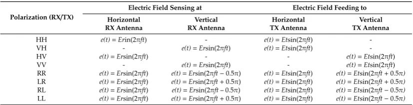
The EM wave feeding from port 1 of the VNA to the TX antennas and from the RX antenna to port 2 of the VNA, and the usage of the phase shifters for every polarization mode are described in Table2 (theoretical) and Table3(practical). Etrepresents the amplitude of the transmitted electric field (at the TX antennas), whereasErrepresents the amplitude of the received electric field (at the RX antennas). Here, the usage ofEt,Er, and the sine function is only to describe the arrangements of phase shifting in the cases of circular polarization. The values ofEtof different measurement cases were not necessarily the same, and the values ofErof different measurement cases were not necessarily the same either.
Table 2. Theoretical wave feeding, wave sensing and phase shifting for linearly polarized (LP) and circularly polarized (CP) modes.
Polarization (RX/TX)
Electric Field Sensing at Electric Field Feeding to Horizontal
RX Antenna
Vertical RX Antenna
Horizontal TX Antenna
Vertical TX Antenna
HH e(t)=Erin(2πft) - e(t)=Etsin(2πft)
-VH - e(t)=Ersin(2πft) e(t)=Etsin(2πft)
-HV e(t)=Ersin(2πft) - - e(t)=Etsin(2πft)
VV - e(t)=Ersin(2πft) - e(t)=Etsin(2πft)
RR e(t)=Ersin(2πft) e(t)=Ersin(2πft−0.5π) e(t)=Etsin(2πft) e(t)=Etsin(2πft+0.5π)
LR e(t)=Ersin(2πft) e(t)=Ersin(2πft+0.5π) e(t)=Etsin(2πft) e(t)=Etsin(2πft+0.5π) RL e(t)=Ersin(2πft) e(t)=Ersin(2πft– 0.5π) e(t)=Etsin(2πft) e(t)=Etsin(2πft−0.5π)
Computation2019,7, 55 9 of 17
Table 3. Practical wave feeding, wave sensing, and phase shifting for LP and CP modes. Please notice the different arrangements of phase shifting for the receiver (RX) right-handed transmitter (TX) right-handed (RR), RX left-handed TX right-handed (LR), RX left-handed TX right-handed (LR), or RX left-handed TX left-handed (LL) modes compared to Table3.
Polarization (RX/TX)
Electric Field Sensing at Electric Field Feeding to Horizontal
RX Antenna
Vertical RX Antenna
Horizontal TX Antenna
Vertical TX Antenna
HH e(t)=Ersin(2πft) - e(t)=Etsin(2πft)
-VH - e(t)=Ersin(2πft) e(t)=Etsin(2πft)
-HV e(t)=Ersin(2πft) - - e(t)=Etsin(2πft)
VV - e(t)=Ersin(2πft) - e(t)=Etsin(2πft)
RR e(t)=Etsin(2πft+0.5π) e(t)=Ersin(2πft) e(t)=Etsin(2πft) e(t)=Etsin(2πft+0.5π) LR e(t)=Ersin(2πft) e(t)=Etsin(2πft+0.5π) e(t)=Etsin(2πft) e(t)=Etsin(2πft+0.5π) RL e(t)=Etsin(2πft+0.5π) e(t)=Ersin(2πft) e(t)=Etsin(2πft+0.5π) e(t)=Etsin(2πft) LL e(t)=Ersin(2πft) e(t)=Etsin(2πft+0.5π) e(t)=Etsin(2πft+0.5π) e(t)=Etsin(2πft)
Please notice that a right-handed circularly polarized (RHCP) TX antenna can be realized by feeding the TX horizontal antenna with a train of sine waves and at the same time feeding the TX vertical antenna with the 90◦
forward-shifted version of the same wave train. Then, upon backscattering by a target, when expecting at the RX antenna, an echo with the same circular direction (RHCP) will be sensed properly if its vertical part (the field sensed by the RX vertical antenna) is shifted 90◦backward before the summation of the horizontal and vertical parts. This is the reason for the phase-shifting direction of the RX vertical antenna being opposite to the TX vertical antenna in the RR case. In the case of LR, the echo received at the RX antenna is expected to have the opposite direction to the transmitted wave, and thus at the RX vertical antenna, the echo is shifted in the same direction as the phase shifting of the TX vertical antenna. This is the main message of Table2.
Unfortunately, the theoretical phase shifting described in Table2requires two types of phase shifters, i.e.,+90◦and−90◦, for realization. When only the same type phase shifters are available for the experiment, then all CP modes can be realized by the technique described in Table3.
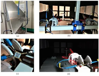
Some activities that took place during the experiment are presented in Figure8, whereas the physical appearances of the targets are depicted in Figure9.
Computation 2019, 7, x FOR PEER REVIEW 9 of 16
Polarization (RX/TX)
Electric Field Sensing at Electric Field Feeding to Horizontal
RX Antenna
Vertical RX Antenna
Horizontal TX Antenna
Vertical TX Antenna
HH e(t) = Ersin(2πft) - e(t) = Etsin(2πft) -
VH - e(t) = Ersin(2πft) e(t) = Etsin(2πft) -
HV e(t) = Ersin(2πft) - - e(t) = Etsin(2πft)
VV - e(t) = Ersin(2πft) - e(t) = Etsin(2πft)
RR e(t) = Etsin(2πft + 0.5π) e(t) = Ersin(2πft) e(t) = Etsin(2πft) e(t) = Etsin(2πft + 0.5π) LR e(t) = Ersin(2πft) e(t) = Etsin(2πft + 0.5π) e(t) = Etsin(2πft) e(t) = Etsin(2πft + 0.5π) RL e(t) = Etsin(2πft + 0.5π) e(t) = Ersin(2πft) e(t) = Etsin(2πft + 0.5π) e(t) = Etsin(2πft) LL e(t) = Ersin(2πft) e(t) = Etsin(2πft + 0.5π) e(t) = Etsin(2πft + 0.5π) e(t) = Etsin(2πft)
Please notice that a right-handed circularly polarized (RHCP) TX antenna can be realized by feeding the TX horizontal antenna with a train of sine waves and at the same time feeding the TX vertical antenna with the 90° forward-shifted version of the same wave train. Then, upon backscattering by a target, when expecting at the RX antenna, an echo with the same circular direction (RHCP) will be sensed properly if its vertical part (the field sensed by the RX vertical antenna) is shifted 90° backward before the summation of the horizontal and vertical parts. This is the reason for the phase-shifting direction of the RX vertical antenna being opposite to the TX vertical antenna in the RR case. In the case of LR, the echo received at the RX antenna is expected to have the opposite direction to the transmitted wave, and thus at the RX vertical antenna, the echo is shifted in the same direction as the phase shifting of the TX vertical antenna. This is the main message of Table 2.
Unfortunately, the theoretical phase shifting described in Table 2 requires two types of phase shifters, i.e., +90° and −90°, for realization. When only the same type phase shifters are available for the experiment, then all CP modes can be realized by the technique described in Table 3.
Some activities that took place during the experiment are presented in Figure 8, whereas the physical appearances of the targets are depicted in Figure 9.
Figure 8. Some activities that took place during the experiment: (a) Measuring the target material’s dielectric constant, (b) after the antenna and the phase shifter installation, (c) the phase shifter, and (d) antenna–target horizontal alignment using a laser liner.
Computation2019,7, 55 10 of 17
Computation 2019, 7, x FOR PEER REVIEW 10 of 16
Figure 9. Targets available for experiments. The cylinder is not part of this report. During the measurement, the bar can be positioned horizontally or vertically.
3. Results
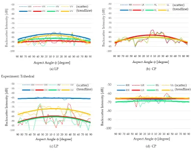
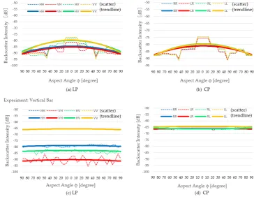
Results of both simulation and experiment are presented here. Through the following graphs, the backscattered EM wave intensity is depicted for each target and each polarization mode. Every figure presents (Figures 10–13) the measurement results of a target where the results of linear polarization and circular polarization can be compared. From the same figure, the simulation results and experimental results of the same target can be compared too. In all figures, the dotted lines are scatter graphs, whereas the solid lines are their second-order polynomial trendlines.
Figure 10. Backscatter intensity of a medium-sized trihedral (w/λ = 6.4): (a) Simulation result of LP, (b) simulation result of CP, (c) experimental result of LP, and (d) experimental result of CP.
Figure 9. Targets available for experiments. The cylinder is not part of this report. During the measurement, the bar can be positioned horizontally or vertically.
3. Results
Results of both simulation and experiment are presented here. Through the following graphs, the backscattered EM wave intensity is depicted for each target and each polarization mode. Every figure presents (Figures10–13) the measurement results of a target where the results of linear polarization and circular polarization can be compared. From the same figure, the simulation results and experimental results of the same target can be compared too. In all figures, the dotted lines are scatter graphs, whereas the solid lines are their second-order polynomial trendlines.
Computation 2019, 7, x FOR PEER REVIEW 10 of 16
Figure 9. Targets available for experiments. The cylinder is not part of this report. During the measurement, the bar can be positioned horizontally or vertically.
3. Results
Results of both simulation and experiment are presented here. Through the following graphs, the backscattered EM wave intensity is depicted for each target and each polarization mode. Every figure presents (Figures 10–13) the measurement results of a target where the results of linear polarization and circular polarization can be compared. From the same figure, the simulation results and experimental results of the same target can be compared too. In all figures, the dotted lines are scatter graphs, whereas the solid lines are their second-order polynomial trendlines.
Figure 10. Backscatter intensity of a medium-sized trihedral (w/λ = 6.4): (a) Simulation result of LP, (b) simulation result of CP, (c) experimental result of LP, and (d) experimental result of CP.
Computation2019,7, 55 11 of 17
Computation 2019, 7, x FOR PEER REVIEW 11 of 16
.
Figure 11. Backscatter intensity of a medium-sized horizontal bar ((l/λ = 6.3, w/λ = 0.4): (a) Simulation result of LP, (b) simulation result of CP, (c) experimental result of LP, and (d) experimental result of CP.
Figure 12. Backscatter intensity of a medium-sized vertical bar ((l/λ = 6.3, w/λ = 0.4): (a) Simulation result of LP, (b) simulation result of CP, (c) experimental result of LP, and (d) experimental result of CP.
Figure 11.Backscatter intensity of a medium-sized horizontal bar ((l/λ=6.3,w/λ=0.4): (a) Simulation result of LP, (b) simulation result of CP, (c) experimental result of LP, and (d) experimental result of CP.
Computation 2019, 7, x FOR PEER REVIEW 11 of 16
.
Figure 11. Backscatter intensity of a medium-sized horizontal bar ((l/λ = 6.3, w/λ = 0.4): (a) Simulation result of LP, (b) simulation result of CP, (c) experimental result of LP, and (d) experimental result of CP.
Figure 12. Backscatter intensity of a medium-sized vertical bar ((l/λ = 6.3, w/λ = 0.4): (a) Simulation result of LP, (b) simulation result of CP, (c) experimental result of LP, and (d) experimental result of CP.
Computation2019,7, 55 12 of 17
Computation 2019, 7, x FOR PEER REVIEW 12 of 16
Figure 13. Backscatter intensity of a medium-sized sphere (d/λ = 6.8): (a) Simulation result of LP, (b) simulation result of CP, (c) experimental result of LP, and (d) experimental result of CP.
4. Discussion
The measurement was done for 64 cases, i.e., two types of test (simulation and experiment), four different targets, and eight different polarization modes. Furthermore, every case was done for 37 different angles. As shown in the figures, for every measurement case, a second-order polynomial trendline was drawn. Despite the opportunity to address many possible comparisons amongst the cases, the obvious trends are discussed here.
4.1. Relationship between Backscatter Intensity and Aspect Angle
A relationship between backscatter intensity and aspect angle happens for the trihedral cases, as shown in [13] and as indicated by the studies in [10,14]. The study in [13] showed proof that the strongest backscatter intensity happens when the EM wave comes from the direction that the trihedral faces (aspect angle = 0°). The studies in [10,14] investigated the effects of trihedral plate damage to the backscatter intensity, but implicitly also showed that, for an ideal trihedral, the strongest backscatter intensity occurs when the EM wave comes from the direction that the trihedral faces direction. The result of our simulation on the trihedral showed agreement with this phenomenon, where the backscatter intensity of most polarization modes returned to the maximum when the aspect angle was around 0°. The simulation resulted in the same trends for the horizontal bar and the vertical bar, where the maximum backscatter intensities happened when the aspect angle was 0°, and the minimum backscatter intensities occurred when the aspect angle was 90°. The same trend was demonstrated consistently for both linear polarization and circular polarization. A different trend was shown in the case of the sphere, where the backscatter intensity graph was flat. This can be explained by the fact that in the simulation we used a perfect sphere model, and this geometry was exactly the same for all aspect angles.
The experiment showed the same trend for most linear polarization modes of the trihedral, horizontal bar, and vertical bar, although with less curving degrees compared to the simulation
Figure 13. Backscatter intensity of a medium-sized sphere (d/λ=6.8): (a) Simulation result of LP, (b) simulation result of CP, (c) experimental result of LP, and (d) experimental result of CP.
4. Discussion
The measurement was done for 64 cases, i.e., two types of test (simulation and experiment), four different targets, and eight different polarization modes. Furthermore, every case was done for 37 different angles. As shown in the figures, for every measurement case, a second-order polynomial trendline was drawn. Despite the opportunity to address many possible comparisons amongst the cases, the obvious trends are discussed here.
4.1. Relationship between Backscatter Intensity and Aspect Angle
Computation2019,7, 55 13 of 17
The experiment showed the same trend for most linear polarization modes of the trihedral, horizontal bar, and vertical bar, although with less curving degrees compared to the simulation results. For the trihedral, the convex curve (maximum atφ=0◦and minimum atφ=90◦) occurred for the VH, HV, and VV cases. For the horizontal bar, the convex curve occurred for the VH and VV cases. For the vertical bar, a less obvious convex curve occurred for the VH and VV cases. The sphere resulted in flat backscatter intensity lines for all linear polarization cases, which was the same as the simulation results.
The results of the experiments for the circular polarization modes unexpectedly differed. All of these cases resulted in a flat curve, meaning that the backscatter intensity value was not related to the aspect angle. The reason for this anomaly is yet unknown and should be subject to further investigation.
4.2. Standard Deviations of CPs and LPs
It is in our interest to understand the behaviors of circularly polarized EM waves when hitting a target. Here, their backscatter intensities were observed at an aspect angle of 0◦
. It was interesting to find that the backscatter intensities of CP modes varied less significantly compared to the backscatter intensities of LP modes. This phenomenon is presented in Table4.
Table 4.Comparison of the standard deviations of CPs and LPs for every target: (a) According to the simulation, and (b) according to the experiment.
(a) Simulation: CP’s vs. LP’s St. Dev. (φ=0◦) (b) Experiment: CP’s vs. LP’s St. Dev. (φ=0◦)
Target
Backscatter Intensity
Standard Deviation (σ) Target
Backscatter Intensity Standard Deviation (σ)
Of All LP Modes Of All CP Modes Of All LP Modes Of All CP Modes
Trihedral 3.00 1.13 Trihedral 8.11 1.30
Horizontal Bar 1.55 0.11 Horizontal Bar 8.88 1.50
Vertical Bar 2.59 0.66 Vertical Bar 8.38 0.91
Sphere 2.09 0.33 Sphere 2.19 0.87
According to the simulation, the standard deviations of CP modes of the trihedral, the horizontal bar, the vertical bar, and the sphere were 1.13, 0.11, 0.66, and 0.33, respectively, which were significantly smaller than the standard deviations of the LP modes, i.e., 3.00, 1.55, 2.59, and 2.09, respectively. The same trend happened in the experiment, where the standard deviations of CP modes of each target were 1.30, 1.50, 0.91, and 0.87, which were significantly smaller than the standard deviations of the LP modes, i.e., 8.11, 8.88, 8.38, and 2.19. This means that the simulation and the experiment show agreement in returning standard deviations for CP modes that are significantly smaller than the standard deviations of LP modes. This phenomenon, in our understanding, can be explained as follows:
• The RX sensor of an LP system employs either a horizontally or vertically polarized antenna, so it
receives only one component of the backscattered waves (either horizontal or vertical). In this way, the values of backscattered wave intensity for each possible mode, i.e., HH, VH, HV, and VV, are potentially significantly different from each other.
• The RX sensor of a CP system employs both horizontally and vertically polarized antennas plus
Computation2019,7, 55 14 of 17
4.3. Backscatter Intensity Differences amongst LP Modes
As discussed in Section4.2, both the simulation and the experiment showed that the standard deviation of the backscatter intensity of linearly polarized EM waves was relatively large. It means that both the simulation and the experiment could differentiate between the backscatter intensities of each HH, VH, HV, and VV case. The details of the variations shown by LP modes (φ=0◦) are presented in Table5, and the details of the CP modes are also presented as a comparison.
Table 5.Backscatter intensity differences amongst LP modes compared to CP modes: (a) Simulation and (b) experiment. Please notice that the backscatter intensities of CP modes varied less significantly compared to LP modes. The ones shaded in green are the largest values of each target for the LP modes.
(a) Simulation: Backscatter Intensity Differences amongst All Polarization Modes (φ=0◦)
Backscatter of LP Modes [dB] Backscatter of CP Modes [dB]
HH VH HV VV St. Dev. RR LR RL LL St. Dev.
Trihedral −81.15 −88.85 −86.22 −82.74 3.00 −83.04 −82.95 −85.37 −85.13 1.13
Horizontal Bar −81.08 −85.38 −83.45 −83.92 1.55 −85.62 −85.70 −85.41 −85.49 0.11
Vertical Bar −84.43 −85.29 −79.89 −79.56 2.59 −80.85 −81.04 −79.55 −79.74 0.66
Sphere −80.54 −76.64 −74.95 −78.50 2.09 −89.56 −89.61 −88.91 −88.94 0.33
(b) Experiment: (a) Backscatter Intensity Differences amongst All Polarization Modes (φ=0◦)
Backscatter of LP Modes [dB] Backscatter of CP Modes [dB]
HH VH HV VV St. Dev. RR LR RL LL St. Dev.
Trihedral −65.39 −84.75 −85.56 −76.79 8.11 −66.53 −65.71 −68.41 −64.93 1.30
Horizontal Bar −65.54 −89.53 −83.98 −80.13 8.88 −65.20 −65.16 −68.67 −65.23 1.50
Vertical Bar −78.80 −88.13 −82.77 −65.47 8.38 −64.53 −66.06 −66.37 −64.29 0.91
Sphere −75.44 −72.92 −70.87 −76.48 2.19 −86.55 −84.60 −84.36 −85.59 0.87
The results of the simulation can be described as the following. For the trihedral, HH returned the largest value (−81.15 dB) whereas VH returned the smallest value (−88.85 dB). For the horizontal bar, HH returned the largest value (−81.08 dB) whereas VH returned the smallest value (−85.38 dB). For the vertical bar, the VV case resulted in the largest value (−79.56 dB) whereas VH resulted in the smallest value (−85.29 dB). For the sphere, HV returned the largest value (−74.95 dB) whereas HH returned the smallest value (−80.54 dB).
The experimental results can be described as the following. For the trihedral, HH returned the largest value (−65.39 dB) whereas HV returned the smallest value (−85.56 dB). For the horizontal bar, HH resulted in the largest value (−65.54 dB) whereas VH resulted in the smallest value (−89.53 dB). For the vertical bar, VV returned the largest value (−65.47 dB) whereas VH returned the smallest value (−88.13 dB). For the sphere, HV returned the largest value (−70.87 dB) whereas VV returned the smallest value (−78.50 dB).