www.nonlin-processes-geophys.net/16/197/2009/ © Author(s) 2009. This work is distributed under the Creative Commons Attribution 3.0 License.
Nonlinear Processes
in Geophysics
Image-model coupling: a simple information theoretic perspective
for image sequences
N. D. Smith1,*, C. N. Mitchell2, and C. J. Budd1
1Department of Mathematical Sciences, University of Bath, BA2 7AY, UK
2Department of Electronic and Electrical Engineering, University of Bath, BA2 7AY, UK
*Completed while with the Department of Electronic and Electrical Engineering, University of Bath, UK
Abstract. Images are widely used to visualise physical
pro-cesses. Models may be developed which attempt to repli-cate those processes and their effects. The technique of cou-pling model output to images, which is here called “image-model coupling”, may be used to help understand the under-lying physical processes, and better understand the limita-tions of the models. An information theoretic framework is presented for image-model coupling in the context of com-munication along a discrete channel. The physical process may be regarded as a transmitter of images and the model as part of a receiver which decodes or recognises those images. Image-model coupling may therefore be interpreted as image recognition. Of interest are physical processes which exhibit “memory”. The response of such a system is not only depen-dent on the current values of driver variables, but also on the recent history of drivers and/or system description. Exam-ples of such systems in geophysics include the ionosphere and Earth’s climate. The discrete channel model is used to help derive expressions for matching images and model out-put, and help analyse the coupling.
Correspondence to: N. D. Smith ([email protected])
1 Introduction
Images describe what is present in a scene, and mathemati-cal or empirimathemati-cal models may be developed which attempt to replicate the underlying processes which produce those im-ages. Given an image, it is interesting to find the model input producing output which best matches the image. In this way useful knowledge concerning the mechanisms producing that image may be discerned. Such image-model coupling, in the context of sequences of images and systems with memory, is described below. The particular example application chosen is the coupling of images of the ionosphere and the output of ionospheric models. This is a challenging problem because the ionosphere (Hargreaves, 2003) is a nonlinear system with regard to the response of its electron content to its driver vari-ables. Furthermore, the system has “memory” since its re-sponse at a given time depends not only on the current drivers but also on the recent history.
There are various questions to consider. What objective function should be used to describe the match between an image sequence and model output? More generally, how can competing models be compared in a quantitative man-ner? And how can the importance of driver variables, for replicating image sequences, be assessed?
of error in coupling model output to images. The objective function used for coupling is statistical in nature; with an in-creased availability of data, it should be possible to derive objective functions which improve the coupling. The context encourages the use of “tools” drawn from information theory and statistical modelling.
The approach borrows heavily from joint source-channel decoding (JSCD), e.g. Garcia-Frias and Villasenor (2001); Ferrari et al. (2005); Link and Kallel (2000) and speech recognition, e.g. Rabiner and Juang (1993), where both maximum a-posteriori (MAP) decoding and evaluation in terms of error rate are commonplace. Modelling channel noise is important for communication systems in general, e.g. Burlina and Alajaji (1998); Beaulieu (1991). Our ap-proach is very similar to the analysis of stochastic channels in Ferrari et al. (2005), except we have here assumed specific conditional independences. This paper seeks to apply con-cepts from information theory and speech recognition to the modelling of geophysical systems; memory is often impor-tant for such systems. The ionosphere (e.g. see Hargreaves, 2003) is used as an illustration in this text. Memory is also important for Earth’s climate, e.g. Maraun et al. (2004). The statistical aspects of our framework are embedded in graph-ical models and the generic Bayesian approach; regarding geophysical systems, note that graphical models, hierarchical Bayesian models and hidden Markov models (HMMs) have previously been applied, e.g. Ihler et al. (2007); Wikle et al. (1998); Beyreuther and Wassermann (2008). There is signif-icant overlap with data assimilation, e.g. Wikle and Berliner (2007); however data assimilation is primarily interested in using models to improve the prediction of observations rather than to decode the values of driver variables. Ignoring this distinction, image-model coupling is essentially a form of data assimilation. Our distinct separation of real-world pro-cess and proposed model is similar to that in Duane et al. (2006), where data assimilation is viewed in terms of the syn-chronisation of two dynamical systems via a noisy communi-cation channel. There are similarities between the framework for data assimilation applied to the ionosphere in Guo et al. (2003) and our approach, but in Guo et al. (2003) there is no development in terms of a discrete communication channel. As far as the authors are aware, the main contribution of this paper is in the application of concepts from JSCD, speech recognition and statistical modelling to the “decoding” of the values of driver variables for geophysical systems, in
partic-ular by highlighting the role of memory and missing vari-ables, and in analysing the coupling. While the concepts are not new, the authors hope the approach may encourage extra insight in modelling geophysical systems.
The paper is organised as follows. First, Sect. 2 introduces discrete channel models with and without memory; the true underlying process producing the image sequence is consid-ered as a transmitter, and the proposed model is part of a receiver which interprets, or decodes, the image sequence. Section 3 then describes the receiver in more detail; the code-book, noise and state transition models, objective function for matching, and the search mechanism. In particular, the assumptions implicit in applying simple sum square error minimisation are detailed. Sections 4 and 5 respectively in-troduce expressions to compare alternative models, and es-timate the sensitivity of image sequences to different driver variables. Finally some discussion and conclusions follow in Sects. 6 and 7.
2 Communication channel framework
true
codebook codebook
proposed RXq
TX
(uTX(t),u′
TX(t))
zTX(t)
(zTX(t),z′
TX(t))
nTX(t)
˜
z(t)
zRXq(t)
nRXq(t)
xRXq(t)
δt
2δt
hcδt
hcδt
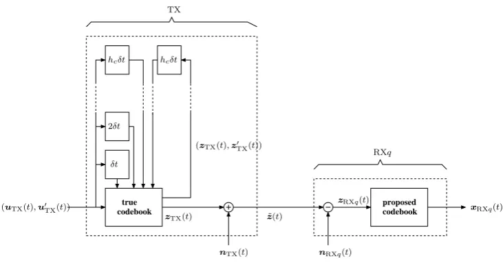
Fig. 1. Image-model coupling as a discrete channel model, where the true real-world process is an encoder,δtis the duration of a timestep when used to describe delay in a temporal buffer, and RXq, q∈{3,2,1}denotes different receivers.
2.1 Transmitter (TX)
Figure 1 describes the true real-world process assumed to generate the images. The process is assumed driven. The driver variables of interest are recorded at timet asuTX(t )∈UTX, whereUTXis a discrete, typically open set1. For the ionosphere, driver variables of interest may include measurements of solar or geomagnetic activity. In addition, there are latent driver variablesu0TX(t )∈UTX0 which are not measured and are typically unknown or not of direct interest to the modeller. Again,
UTX0 is a discrete set. The current system is fully described byzTX(t )∈ZTX andz0TX(t )∈Z 0
TX, which respectively describe those variables which form the image, and the complementary set of variables required to complete the full description. For convenience, define discrete sets ZTX⊆Z andZ0TX⊆Z0. The real-world process is assumed viewed as a codebook which implements the deterministic mapping, for some fixed and known channel memory length2 hc∈N0 (for channel memory, e.g. see Khinchin, 1957),
zTX(t ):(uTX(t−hc, t ),u0TX(t−hc, t ),zTX(t−hc),z0TX(t−hc))7→zTX(t ), (1) wheretis the timestep index andhcis expressed in timesteps, and for example,
uTX(t−hc, t )≡(uTX(t−hc),uTX(t−hc+1), . . . ,uTX(t )).
Similar abbreviations are used elsewhere for time-ordered temporal sequences of vectors. HencezTX(t )is fully determined by the present and past driver variables, both known and latent, and an initial complete description. Hence there are no variables beyond those in the domain of the mapping which cause variation inzTX(t ). The assumption of the deterministic mapping is thought reasonable due to the inclusion of all driver variables and description variables in the domain. In the case of the ionosphere, the dependency on initialisation is assumed since the ionosphere is not memoryless; its description may evolve differently over time under the action of the same sequence of drivers depending on the initial distribution of plasma.
There is also memory in the source. Lettinghs∈N0denote the length of source memory in timesteps, then it is convenient to define the state,
xTX(t )=(uTX(t−h, t ),u0TX(t−h, t ),zTX(t−h),z0TX(t−h)), (2)
whereh=max[hs−1, hc], wherexTX(t )∈XTX, and whereXTX=(⊗hi=1+1UTX)(⊗hi=1+1U 0
TX)⊗ZTX ⊗ZTX0 . This definition of state allows the transmitter to be modelled as a hidden Markov process (see Sect. 3.4).
1The constraint of discrete signals and sets rather than continuous analogues is necessary for a discrete channel model; although real-world processes are typically continuous, discretisation may be regarded as the result of sampling continuous signals or spaces into the machine precision of the recording, storage or computing device.
2The notation
The actual image measured or recorded at timet isz(t )˜ ∈Z. This image is related to the partial descriptionzTX(t )by, ˜
z(t )=zTX(t )+nTX(t ), (3)
wherenTX(t )∈Zis additive noise describing error in the measuring devices. Unfortunately, if an image is incomplete, it is sometimes necessary to complete the image, for example using tomographic reconstruction. For the purposes of this analysis, such images are regarded as if directly imaged by a device, and the error in the reconstruction included into the noise process
nTX(t ). Both the true real-world process and noise source may be nonstationary; however for the estimation of the statistical models described later, properties of stationarity and ergodicity (Korn and Korn, 1968) are convenient. The noise signal
nTX(t )is not transmitted independently along the channel, only the image z(t )˜ . In practice, it is usual to consider a finite length sequence of images, for exampleT imagesz(˜ 1, T ).
2.2 Level 3 receiver (RX3)
With infinite knowledge, it is possible to construct a receiver which implements the reverse process to the transmitter. Hence the receiver first “denoises” the image,
zRX3(t )= ˜z(t )−nRX3(t ), (4)
wherenRX3(t )∈Z,zRX3(t )∈ZRX3, and ZRX3 is typically a discrete set denoting the range of the receiver codebook. The codebook implements deterministic mappings of form,
zRX3(t ):(uRX3(t−hc, t ),u0RX3(t−hc, t ),zRX3(t−hc),z0RX3(t−hc))7→zRX3(t ), (5) but is used in the reverse direction. The codebook is typically implemented by a deterministic mathematical or empirical model. The noise sourcenRX3(t )should model the measurement noise in the imaging devices. This receiver is unrealisable, but is included since it permits decoding with the lowest possible error rate. Decoding is described more fully in Sect. 3.4. For clarity, the receiver is here called a level 3 receiver, where the higher the level, the deeper the conditional dependencies in the receiver codebook. For convenience, a receiver state is defined,
xRX3(t )=(uRX3(t−h, t ),u0RX3(t−h, t ),zRX3(t−h),z0RX3(t−h)), (6)
whereh=max[hs−1, hc]andxRX3(t )∈XRX3=(⊗hi=1+1URX3)(⊗hi=1+1URX30 )⊗ZRX3⊗ZRX30 . 2.3 Level 2 receiver (RX2)
This is similar to the level 3 receiver with differences in the codebook mappings and notation. Denoising is,
zRX2(t )= ˜z(t )−nRX2(t ), (7)
wherenRX2(t )∈ZandzRX2(t )∈ZRX2. The codebook implements deterministic mappings of form,
zRX2(t ):(uRX2(t−hc, t ),zRX2(t−hc, t−1))7→zRX2(t ), (8)
where the unmeasured or unknown driver and description variables inUTX0 andZTX0 have been omitted. The stochastic variation inz(t )˜ due to these variables is instead incorporated into a more complicated noise sourcenRX2(t ). The noise source no longer models the error in measurement devices alone, but also the stochastic variation due to the omitted variables. Again, define a state,
xRX2(t )=(uRX2(t−h, t ),zRX2(t−h, t−1)), (9)
whereh=max[hs−1, hc], andxRX2(t )∈XRX2 =(⊗hi=1+1URX2)(⊗hi=1ZRX2). 2.4 Level 1 receiver (RX1)
This is similar to the level 3 and 2 receivers with differences in the codebook mappings and notation. Denoising is,
zRX1(t )= ˜z(t )−nRX1(t ), (10)
wherenRX1(t )∈ZandzRX1(t )∈ZRX1. The codebook implements deterministic mappings of form,
zRX1(t ):uRX1(t )7→zRX1(t ). (11)
Each codebook entryzRX1(t )may be regarded as “typical” for its driver variables, in a similar manner to which the mean of a Gaussian distribution is typical of samples drawn from that Gaussian. The noise sourcenRX1(t )should now also describe the stochastic variation due to different initialisations and histories of driver variables. The present drivers form the state so
2.5 Perfect image-model coupling
In this analysis, perfect image-model coupling is the transmission of a sequence of driver variables, without loss, via the true real-world process as encoder, the images as the transmitted message, and the proposed model as part of the decoder. Ideally
uTX(t )=uRXq(t ). For the example of the level 3 receiver, assume that,
– the codebook mappings are identical, i.e.z−1RX3(t )◦zTX(t )=I, whereI is the identity map,
– the domain of the receiver and transmitter codebooks are identically descriptive, i.e.URX3=UTX,
– the transmitter noise source is correctly modelled by the receiver noise source, i.e.PRX3(nRX3(t ))=PTX(nTX(t )),∀t, and,
– processes and models implicit in the transmitter and receiver are assumed stationary.
The first two conditions assume the proposed codebook is correct, the third that the noise model is correct. Unfortunately, even under these conditions where the distribution of noisenRX3(t )is correct, the particular sample drawn from that noise distribution remains unknown. For this reason, even in the case of the level 3 receiver, perfect coupling may not be achievable. In many cases, the driver variables uTX(t )can only be recovered in the sense of maximum a-posteriori (MAP) or other estimates. For either of the level 3, 2 or 1 receivers, perfect coupling would only be possible if the transmitter and receiver were identical, and either noise samples were transmitted independently between the transmitter and receiver along a separate noiseless channel, or the supports of the noise distributions were always strictly less than the distances between neighbouring entries in the ranges of the transmitter and receiver codebooks. Decoding is described more fully in Sect. 3.
3 Receiver
The purpose of the receiver is to decode the image sequencez(˜ 1, T )as a sequence of driver variables. Assume the receiver at levelqimplements this by first decoding the most appropriate state sequence through minimising a scalar objective function,
ˆ
xRXq(1, T )(z(˜ 1, T ))=argxRXq(1,T )∈⊗Tt=1XRXqminfRXq(xRXq(1, T ),
˜
z(1, T )), (12)
subject to the constraint that there exists an underlying consistent driver sequence uˆRXq(1, T )(z(˜ 1, T )), i.e. an extraction
mapping should exist, ˆ
xRXq(1, T )(z(˜ 1, T ))7→ ˆuRXq(1, T )(z(˜ 1, T )). (13)
This section explains how the receiver achieves this. The definition of the receiver requires the specification of (1) a codebook, both the mapping as implemented by a deterministic model and its domain, (2) a noise model, and (3) a state transition model. The decoder attempts to find the best match between each image and a member of the codebook. This requires careful selection of (4) the objective function to measure the “goodness of match”, and (5) a search mechanism, often heuristic, to navigate the codebook and find the member with maximum “goodness of match”. These components are described in the remainder of this section.
3.1 Codebook
For the levelqreceiver, the codebook may be viewed as the set of deterministic mappings,
CRXq = {xRXq(t )7→zRXq(t ),∀xRXq(t )∈XRXq}. (14)
These may be implemented using lookup tables, but more typically by empirical or mathematical models. The codebook domainXRXqmay also be constrained by the choice of model. For example an empirical model may impose lower and upper
3.2 Noise model
Since the codebook is deterministic, stochastic variability must be introduced via a supplementary noise model. For the level
qreceiver, the noise process may be fully specified via a set of probability mass functions (PMFs),
NRXq= {PRXq(nRXq(t )|xRXq(t )),∀nRXq(t )∈Z,∀xRXq(t )∈XRXq}. (15)
In effect{CRXq,NRXq}defines a stochastic version of the deterministic codebook. Indeed if the model involved in
image-model coupling is stochastic, then there is no need to defineCRXqandNRXqseparately. Ideally the codebook and noise model
should replicate the stochastic variation in the transmitter (i.e. the real-world process). However this is a challenging task since considerable complexity is expected in the real-world variation, as described in Appendix A.
3.3 State transition model
Another supplementary model must be supplied governing the transitions between consecutive states. This may again be fully specified by a set of PMFs. For a levelqreceiver,
ARXq = {PRXq(xRXq(t )|xRXq(t−1)),∀xRXq(t )∈XRXq,∀xRXq(t−1)∈XRXq}. (16)
This state transition model must assign zero probability mass to those transitions which do not respect a temporally consistent sequence, e.g. foruRXq(1, T ).
3.4 Objective function
The objective function should be derived from a decision theoretic perspective. For each samplez(˜ 1, T ), the decision rule should seek to minimise the conditional risk (Duda et al., 2001),
R(xRXq(1, T )| ˜z(1, T ))=
X
yRXq(1,T )∈⊗Ti=1XRXq
l(xRXq(1, T ),yRXq(1, T ))PRXq(yRXq(1, T )| ˜z(1, T )), (17)
wherexRXq(t )∈XRXq,∀t∈[1, T]. The scalar functionl(·,·)is the loss, and the conditional risk is expressed as the average
loss over a posterior distribution in the receiver. An intuitive choice of loss function is the squared L2 norm of the difference between the two arguments. However, under such a “regression-based” loss, the conditional risk is expensive to compute if samples must be drawn from the posterior. A simpler “classification-based” loss may instead be used (Duda et al., 2001),
l(xRXq(1, T ),yRXq(1, T ))=
0 ifxRXq(1, T )=yRXq(1, T )
1 otherwise . (18)
This is preferable because it reduces computational cost since then,
R(xRXq(1, T )| ˜z(1, T ))=1−PRXq(xRXq(1, T )| ˜z(1, T )), (19)
thereby avoiding the averaging operation. Hence an objective function may be expressed as follows, where logs are taken and unneccessary terms are discarded from the log posterior,
fRXq(xRXq(1, T ),z(˜ 1, T ))= −lnPRXq(z(˜ 1, T )|xRXq(1, T ))−lnPRXq(xRXq(1, T )). (20)
The first of the two terms in the objective function models state-dependent noise, the second models memory in the state space (which includes memory in the driver source). Stochastic variation originates both in the channel and the source (e.g. see Khinchin, 1957). The first term is determined by the codebookCRXqand noise modelNRXq, the second by the state transition
modelARXq. The resultant decoder is the well-known maximum a-posteriori (MAP) decoder where the posterior acts as a
xRXq(t) zRX
q(t)
˜
z(t)
nRXq(t)
xRXq(t+ 1) zRX
q(t+ 1)
˜
z(t+ 1)
nRXq(t+ 1)
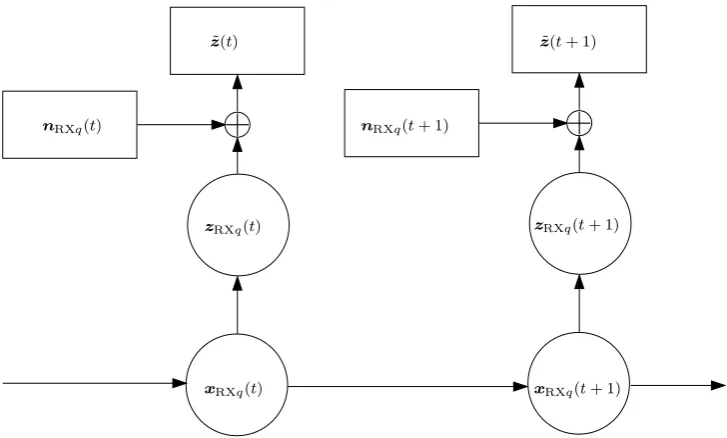
Fig. 2. Temporal portion of hidden Markov model (HMM) for modelling the receiver RXq,q∈{3,2,1}.
3.4.1 Discrete channel with memory
All receivers RXq,q∈{3,2,1}may be modelled as hidden Markov processes of the form shown in Fig. 2, where the state is assumed to contain all information about the past which can influence the present and the future.
The noise process and state transition process are assumed stationary in time. The posterior is,
PRXq(xRXq(1, T )| ˜z(1, T ))= QT
t=1PRXq(z(t )˜ |xRXq(t ))PRXq(xRXq(t )|xRXq(t−1)) PRXq(z(˜ 1, T ))
, (21)
where it is assumed that the statexRXq(0)is fully known, i.e. the history of driver variables and pre-noised images is known
back to a timestep index of−h, if required. The objective function becomes,
fRXq(xRXq(1, T ),z(˜ 1, T ))= − T X
t=1
{lnPRXq(z(t )˜ |xRXq(t ))+lnPRXq(xRXq(t )|xRXq(t−1))}. (22)
Both level 3 and level 2 receivers assume channel memory length and source memory length no greater than h andh+1 timesteps respectively. Of course, those memory lengths may in practice be reduced by constraining the PMFs inNRXq and
ARXq. For example, channel memory length may be reduced to zero in favour of source memory alone.
3.4.2 Discrete memoryless channel
The discrete memoryless channel is well known and is worthy of further consideration. Assume the probability of a state is independent of the previous state. This is not possible for a level 3 or 2 receiver. For the level 1 receiver,
fRX1(uRX1(1, T ),z(˜ 1, T ))= −
T X
t=1
with time. The ionosphere’s response, as illustrated by its description, under the action of a given set of drivers, will vary depending on its past driver values. However the discrete memoryless assumption is convenient and, at the risk of reduced decoding accuracy, the likelihoodPRX1(z(t )˜ |uRX1(t ))may be regarded as averaged over all possible histories.
3.4.3 Discrete memoryless channel with state-independent Gaussian noise
The objective function for the discrete memoryless channel, as given in Eq. (23), may be simplified to yield the well-known sum square error and sum weighted square error objective functions. It is useful to consider the additional assumptions.
First, it is sometimes convenient to assume that the mappinguRX1(t )7→zRX1(t )is injective∀t∈[1, T](e.g. see “Mappings” by I. N. Sneddon in Sneddon, 1976). The injective assumption may not be unreasonable, particularly when a vector of few driver variables maps into a large image with many components. Then the objective function in Eq. (23) becomes,
fRX10 (uRX1(1, T ),z(˜ 1, T ))= −
T X
t=1
{lnPRX1(z(t )˜ |zRX1(t ))+lnPRX1(uRX1(t ))}. (24)
The priorPRX1(uRX1(t ))should reflect the frequency of occurrence of different values of driver variables over all possible histories. For example, for the ionosphere the prior may be calculated using measurements collected over a full solar cycle.
Next consider the noise process is state-independent and is stationary in time. Hence PRX1(z(t )˜ |zRX1(t )) = δ(z(t )˜ −
zRX1(t ),nRX1)PRX1(nRX1), where δ(·,·) is the Kronecker delta, simplifying the noise model NRX1 considerably to the specification of a single PMF. This is unlikely for systems such as the ionosphere. Additionally, assume the noise model is a zero-mean discretised Gaussian so PRX1(nRX1) = N (nRX1;0,R) where R is the covariance matrix3, and hence
PRX1(z(t )˜ |zRX1(t ))=N (z(t )˜ ;zRX1(t ),R). Unfortunately, Gaussianity is unlikely for those description variables, for example line integrals of electron content in the case of the ionosphere, which are naturally nonnegative.
Finally, assume there is no prior preference in the driver variables so there is a uniform priorPRX1(uRX1(t ))overURX1. Again this is probably unreasonable for many real-world systems. For the case of the ionosphere, quiet space weather occurs much more frequently than stormy space weather, and the prior over driver variables should reflect this. The objective function for the discrete memoryless channel in Eq. (24) may now be simplified to the following, where irrelevant terms have been discarded,
fRX100 (uRX1(1, T ),z(˜ 1, T ))=
T X
t=1
zRX1(t )>R−1( 1
2zRX1(t )− ˜z(t )). (25)
The more negative the objective function, the better is the “goodness of match”. If the covariance matrix R is assumed diagonal, minimisation is equivalent to the conventional least sum weighted square error solution. The diagonal elements, i.e. weights, represent the relative “importance” of each component in the image. If each component is of equal importance, R may be set to Identity and the minimisation yields the least sum square error solution.
3.5 Search
Minimisation of the objective function over the full domain⊗T
t=1XRXqof the receiver codebook requires a search mechanism. The simplest approach is full grid search. However computational cost increases with the number of state variables, and coarser grid searches must often be introduced. Otherwise conventional derivative-based optimisation is recommended. However if the codebook mapping is implemented by some deterministic empirical model or when a mathematical model is very complicated, the derivative of an objective function of typefRXq(·)may not be known analytically. In this case, derivative-free optimisation
techniques may then be required. Alternative approaches include numerical approximation of gradients (e.g. see the algorithms in Powell, 2007) and sampling-based methods. An example of a sampling scheme is simulated annealing (Salamon et al., 2002) which, although it converges to a global minimum, requires many evaluations of the objective function. A variant of simulated annealing is fast annealing (Salamon et al., 2002). Further comments on decoders are given in Sect. 6.
4 Evaluation
It is sometimes useful to compare different codebooks for image-model coupling. Codebooks should not be compared in isolation, but in the context of the accompanying noise model, state transition model, objective function and search mechanism.
The error rate associated with each full receiver is the risk (Duda et al., 2001),
E(RXq)= X
˜
z(1,T )∈⊗T t=1Z
R(xˆRXq(1, T )| ˜z(1, T ))PTX(z(˜ 1, T )), (26)
with the conditional risk as given in Eq. (17) under the loss as given in Eq. (18). If each levelq receiver is correct such thatMRXq={CRXq,NRXq,ARXq}exactly replicates the statistical properties of the transmitter under the constraints imposed
within each receiver, then E(RX3)≤E(RX2)≤E(RX1). This relationship does not necessarily hold for incorrect receivers. Indeed when all receivers are incorrect, simpler receivers can often prove more robust and give lower error rates in practice.
However the error rate penalises the decoding of variables, with values which differ from those in the transmitter, with the same loss independent of the degree of difference. This may be misleading. An alternative quantity is the mutual information between the sequence of true driver variablesuTX(1, T )and the sequence of received driver variablesuRXq(1, T ). Perfect
coupling, or lossless transmission, maximises this quantity. Any attempt to improve, learn or adapt incorrect models should aim to increase this quantity. Using MacKay (2004), the mutual information may be expressed as,
I (uRXq(1, T );uTX(1, T ))=H (uTX(1, T ))−H (uTX(1, T )|uRXq(1, T )), (27)
where the first and second terms on the right hand side are respectively source and conditional entropies. Since the source entropy is assumed fixed, the following simpler quantity may instead be used. Using MacKay (2004) for the expression for conditional entropy,
F (MRXq)= −H (uTX(1, T )|uRXq(1, T ))
= X
uRXq(1,T )∈⊗Tt=1URXq
PRXq(uRXq(1, T ))
X
uTX(1,T )∈⊗Tt=1UTX
P (uTX(1, T )|uRXq(1, T ))lnP (uTX(1, T )|uRXq(1, T )), (28)
where,
−H (uTX(1, T ))≤F (MRXq)≤0. (29)
Note that some form of mutual information decoding would be more compatible with this comparison scheme, but MAP decoding simplifies the implementation of decoders. Rearranging and introducing the latent variablesz(˜ 1, T ),
F (MRXq)=
X
uRXq(1,T )∈⊗Tt=1URXq
X
˜
z(1,T )∈⊗T t=1Z
X
uTX(1,T )∈⊗Tt=1UTX
P (uRXq(1, T ),z(˜ 1, T ),uTX(1, T ))
lnP (uTX(1, T )|uRXq(1, T )). (30)
Making some conditional independence assumptions reasonable for our communication channel,
F (MRXq)=
X
uRXq(1,T )∈⊗Tt=1URXq
X
˜
z(1,T )∈⊗Tt=1Z
X
uTX(1,T )∈⊗Tt=1UTX
PRXq(uRXq(1, T )| ˜z(1, T ))
PTX(z(˜ 1, T )|uTX(1, T ))PTX(uTX(1, T ))lnP (uTX(1, T )|uRXq(1, T )). (31)
Unfortunately it is difficult to estimate the distributions defined on the transmitter variables. However for the level 1 receiver, the quantity may be approximated by assuming the transmitter and receiver codebook mappings are injective (e.g. see “Mappings” by I. N. Sneddon in Sneddon, 1976) and the noise processnTX(t )is negligible. Thenz(t )˜ ≈zTX(t ),∀t∈[1, T]. Drawing` samples of typeuTX(1, T )according to the priorPTX(uTX(1, T ))then,
F (MRX1)≈ 1
` ` X
l=1
X
zRX1(1,T )∈⊗Tt=1ZRX1
PRX1(zRX1(1, T )| ˜zl(1, T ))lnPRX1(z˜l(1, T )|zRX1(1, T )), (32)
where z˜l(1, T ) is injectively mapped through the transmitter codebook from the lth sample drawn according to PTX(uTX(1, T )). Ignoring all posterior probability mass not located at the decoded solution,
F (RX1)≈ 1
` ` X
l=1
PRX1(zˆRX1(1, T )| ˜zl(1, T ))lnPRX1(z˜l(1, T )| ˆzRX1(1, T )), (33)
algorithm. In the context of ionospheric modelling, each of the `samples may be a sequence collected from a different day’s data. When`is small, alternative quantities which also penalise model complexity should be considered, for example stochastic complexity (e.g. see Gr¨unwald et al., 2005). It is difficult to evaluate a receiver based on a single sample, i.e. when
`=1, though useful insight may still be possible.
Continuing with the level 1 receiver, as in Sect. 3.4 assume the noise process for the memoryless channel is state-independent, zero-mean discretised Gaussian and stationary in time. Then,
F (RX1)≈ 1
` ` X
l=1
T Y
t=1
PRX1(zˆRX1(t )| ˜zl(t )) T X
t=1
lnPRX1(z˜l(t )| ˆzRX1(t )), (34)
where,
PRX1(zˆRX1(t )| ˜zl(t ))=
PRX1(z˜l(t )| ˆzRX1(t ))PRX1(zˆRX1(t ))
P
zRX1∈ZRX1PRX1(z˜l(t )|zRX1)PRX1(zRX1)
, (35)
andPRX1(z˜l(t )| ˆzRX1(t ))=N (z˜l(t ); ˆzRX1(t ),R).
5 Sensitivity
Sensitivity of a sequence of true imageszTX(1, T )to the different state variables, including driver variables, inxTX(1, T )is of scientific interest. For example, during a geomagnetic storm, what drivers are most influential in producing the particular electron content patterns in the ionosphere? If the true real-world process is nonlinear, sensitivity must typically be evaluated at each sequence of state variables of interest. At the state sequenceyTX(1, T ), the Fisher information (see “Fisher information” in Wikipedia, access: October 2008) is,
Jij(yTX(1, T ); {CTX,ATX})=
X
zTX(1,T )∈⊗Tt=1ZTX
δ2lnP (zTX(1, T )|xTX(1, T ))
δ[xTX(1, T )]iδ[xTX(1, T )]j
x
TX(1,T )=yTX(1,T )
PTX(zTX(1, T )|xTX(1, T ))|xTX(1,T )=yTX(1,T ), (36)
where[xTX(1, T )]iis theith component in the sequence of state variables, and{CTX,ATX}refers to the real-world process. Re-lating to drivers,δdenotes discrete differences but under the assumption that all values in the relevant component inxTX(1, T ) are uniformly spaced. Since the true images are unknown,
Jij(yTX(1, T ); {CTX,ATX})≈Jij(yTX(1, T );MTX)
= X
˜
z(1,T )∈⊗Tt=1Z
δ2lnP (z(˜ 1, T )|xTX(1, T ))
δ[xTX(1, T )]iδ[xTX(1, T )]j
x
TX(1,T )=yTX(1,T )
PTX(z(˜ 1, T )|xTX(1, T ))|xTX(1,T )=yTX(1,T ). (37)
Unfortunately, the transmitter distributions are also unknown, but the Fisher information may be approximated at the receiver,
Jij(yTX(1, T );MTX)≈Jij(yRXq(1, T );MRXq)
= X
˜
z(1,T )∈⊗T
t=1Z
δ2lnPRXq(z(˜ 1, T )|xRXq(1, T )) δ[xRXq(1, T )]iδ[xRXq(1, T )]j
x
RXq(1,T )=yRXq(1,T )
PRXq(z(˜ 1, T )|xRXq(1, T ))|xRXq(1,T )=yRXq(1,T ). (38)
The Fisher information defined upon the receiver is subject to the receiver’s statistical assumptions, and may be a poor ap-proximation to that defined on the transmitter. Since the Fisher information is defined onMRXq, it does not depend on the
optimisation algorithm. In terms of the objective function, and assumingPRXq(xRXq(1, T ))is uniform,
Jij(yRXq(1, T );MRXq)= − X
˜
z(1,T )∈⊗Tt=1Z
δ2fRXq(z(˜ 1, T ),xRXq(1, T )) δ[xRXq(1, T )]iδ[xRXq(1, T )]j
xRXq(1,T )=yRXq(1,T )
Given a single samplez˜l(1, T )and a level 1 receiver, a possible estimate at sequencevRX1(1, T )is,
Jij(vRX1(1, T );MRX1)≈ −
δ2fRX1(z˜l(1, T ),uRX1(1, T ))
δ[uRX1(1, T )]iδ[uRX1(1, T )]j
u
RX1(1,T )=vRX1(1,T )
, (40)
notingxRX1(1, T )=uRX1(1, T ). In this case the Fisher information is estimated using the negative Hessian of the objective function. However such an estimate may be misleading since it is “tuned” to one particular image sequence only, i.e. all the conditional probability mass for observed sequences is assumed located atz˜l(1, T ).
6 Discussion
The selection of driver and image variables for URXq and Z respectively is critical. If the selection is not sufficiently descriptive, then the noise distributions implied in the trans-mitter may be very broad due to the effect of latent variables. Essentially, too much useful information may then be lost in the encoding process. Unfortunately, the choice of vari-ables is often restricted by the particular receiver codebook, e.g. empirical or mathematical model, used.
In designing the receiver, the codebook is intuitively most important and effort should first be directed at improving this. The choice of noise model and state transition model should be data-dependent, since they should be learnt from data. This influences the choice of objective function and level of receiver. The simpler receivers should be more ro-bust if there is a lack of good quality data. However it is important to understand the assumptions implicit in the sim-pler receivers, especially regarding the conditional indepen-dences. Of course, the level 3 and level 2 receivers reduce to the level 1 receiver if the level 1 assumptions hold in the transmitter. The choice ofhs,hcandhmay be driven by
lim-itations in data rather than scientific knowledge. The inverse problem of decoding state variablesxˆRXq(1, T )for a noisy
image sequencez(˜ 1, T )has a unique solution providing the objective function has a single global minimum.
The receiver codebook has been defined using a single deterministic model. However multiple models may be used in parallel where the data fusion occurs at the level of
zRXq(1, T )or xRXq(1, T ). For ionospheric modelling, the
fusion may additionally use geographic information where alternative ionospheric models are weighted differently at different global locations, for example according to their ability to model low latitude or polar/auroral processes.
The approach described above is limited. Our HMM en-forces specific conditional dependencies; it is possible to ap-ply different graphical models, e.g. Ihler et al. (2007). For example, the PMFs in our approach may be further con-strained by incorporating spatial dependencies between vari-ables, such as between pixels in an image, e.g. Burlina and Alajaji (1998); Link and Kallel (2000). When the channel is not memoryless, our approach also assumes additive Markov noise; other noise models are possible, for example semi-Markov noise (e.g. Chvosta and Reineker, 1999), or nonad-ditive noise. The approach is able to model intersymbol inter-ference (ISI), as explained in Ferrari et al. (2005). It can also
model the finite-state Markov channel (FSMC), e.g. Gold-smith and Varaiya (1996); Li and Collins (2007), where the driver variables form the system input. Implementing the de-coder is challenging; a possible implementation is the Viterbi algorithm, e.g. Rabiner and Juang (1993); Kavˇci´c and Moura (2000). However in practice, decoders may be too compu-tationally expensive to implement unless the codebook map-ping is computed apriori and stored in lookup tables, or the codebook mapping is very simple. Regarding decoders, it may be possible to incorporate concepts from JSCD such as interleavers, e.g. Li and Collins (2007), and the decoding al-gorithm, linked to Baum-Welch estimation, in Garcia-Frias and Villasenor (2001). Generally, it is difficult estimating PMFs with limited data, though concepts from speech recog-nition such as state and mixture tying and language model smoothing, e.g. Rabiner and Juang (1993), may prove ben-eficial. The accurate estimation of PMFs in the noise and state transition models is the main drawback of this approach. In practice, many simplifications may be required, in which case the receiver may degrade to a much simpler form. As detailed in Maraun et al. (2004), memory is often associated with the correlation function, and may be finite or infinite. It would be useful to analyse our approach by relating it to such a definition of memory.
Similar “receivers” have been developed in nonlinear and linear time series analysis. Examples from nonlinear time series analysis include the non-linear autoreggresive (NLAR) model (Chatfield, 2004), non-linear moving aver-age (NLMA) model (Tong, 1990) and state-dependent model (SDM) (Priestley, 1988); however these examples assume there is no hidden state, equivalent to there being no chan-nel noise. Also, Variable order Markov Models (VMMs) (Begleiter et al., 2004) model memory, but again there are no hidden states. The ARMA-filtered hidden Markov model (Michalek et al., 2000) may possibly be regarded as a special case of the level 2 receiver, at least in concept.
as the image, but the resolution is too coarse, the ability of the receiver to “recognise” small-scale structures is inhibited. Image-model coupling is simply an attempt to recognise or classify an image in terms of its driver variables.
7 Conclusions
Presented above is an information theoretic framework de-scribing image-model coupling when the true-world system has memory. Examples of such systems include the iono-sphere and other geophysical systems with a “sluggish re-sponse”. A discrete channel model is used to help quantify the match between images and model output, and analyse the coupling. The approach is statistical in nature. It should be
possible to harness any increased availability of data to de-rive objective functions which better reflect the spatial and temporal statistical relationships in the true underlying pro-cess, and thereby improve coupling as measured by decoding error rate. However for complex systems such as the iono-sphere it is probably more beneficial to first direct effort at improving the accuracy of the proposed model (i.e. the code-book). It is hoped that the framework described above may encourage the further use of statistical and information-based “tools” in image-model coupling and its analysis. In general, image-model coupling may be used to help us better under-stand the underlying processes which produce the effects be-ing imaged, but also better understand the limitations of our proposed models too.
Appendix A
Distributions implicit in the transmitter
The noisy imagez(t )˜ may be regarded as sampled from a distribution, the functional form of which varies with the number of conditional variables. An expression for the fully marginalised distributionPTX(z(t )˜ |uTX(t ))may be derived under the following assumptions, consistent with the transmitter illustrated in Fig. 1.
– InUTX⊗UTX0 , each driver variable is linearly independent of all other driver variables.
– InZ⊗Z0, each description variable is linearly independent of all other description variables.
– Measurement noise is stationary temporally and is state-independent. HencePTX(nTX(t )|zTX(t ))=PTX(nTX)∀zTX(t ),∀t.
– The pre-noised imagezTX(t )is fully determined by an initialisationhctimesteps previous wherehc∈N0, and the history
of driver variables since then, so,
(uTX(t−hc, t ),u0TX(t−hc, t ),zTX(t−hc),z0TX(t−hc))7→zTX(t ). (A1)
If no such value ofhcexists, then a value ofhcis chosen such that the history of driver variables prior to timestep(t−hc)
has no significant effect on the likelihood of the current description given the full description att−hc.
So,
PTX(z(t )˜ |uTX(t−hc, t ),u0TX(t−hc, t ),zTX(t−hc),z0TX(t−hc))=PTX(nTX)δ(nTX,z(t )˜ −zTX(t )), (A2)
whereδ(·,·)is the Kronecker delta. Introducing redundant variables into the list of conditional variables,
PTX(z(t )˜ |uTX(t−hc, t ),u0TX(t−hc, t ),zTX(t−hc, t ),z0TX(t−hc, t ))
Marginalising over the unknown description and driver variables, and substituting from above,
PTX(z(t )˜ |uTX(t−hc, t ),zTX(t−hc, t ))
= X
u0
TX(t−hc,t )∈⊗hc +1 i=1 U
0 TX
X
z0
TX(t−hc,t )∈⊗hc +1 i=1 Z
0 TX
PTX(u0TX(t−hc, t ),z0TX(t−hc, t ))
PTX(z(t )˜ |uTX(t−hc, t ),u0TX(t−hc, t ),zTX(t−hc, t ),z0TX(t−hc, t ))
= X
u0
TX(t−hc,t )∈⊗hci=+11U 0 TX
X
z0
TX(t−hc,t )∈⊗hci=+11Z 0 TX
PTX(nTX)δ(nTX,z(t )˜ −zTX(t ))
[
hc−1 Y
a=0
PTX(z0TX(t−a)|z 0
TX(t−hc, t−a−1),u0TX(t−hc, t ))]
PTX(z0TX(t−hc)|u0TX(t−hc, t ))[ hc−1
Y
a=0
PTX(u0TX(t−a)|u 0
TX(t−hc, t−a−1))]PTX(u0TX(t−hc)). (A4)
Then,
PTX(z(t )˜ |uTX(t ))
= X
uTX(t−hc,t−1)∈⊗hci=1UTX
X
zTX(t−hc,t )∈⊗hc +1 i=1 ZTX
PTX(z(t )˜ |uTX(t−hc, t ),zTX(t−hc, t ))
PTX(uTX(t−hc, t−1),zTX(t−hc, t ))
= X
uTX(t−hc,t−1)∈⊗hci=1UTX
X
zTX(t−hc,t )∈⊗hci=+11ZTX
PTX(z(t )˜ |uTX(t−hc, t ),zTX(t−hc, t ))
[
hc−1 Y
a=1
PTX(zTX(t−a)|zTX(t−hc, t−a−1),uTX(t−hc, t−1))]
PTX(zTX(t )|zTX(t−hc, t−1),uTX(t−hc, t−1))PTX(zTX(t−hc)|uTX(t−hc, t−1))
[
hc−1 Y
a=1
PTX(uTX(t−a)|uTX(t−hc, t−a−1))]PTX(uTX(t−hc)), (A5)
wherePTX(z(t )˜ |uTX(t−hc, t ),zTX(t−hc, t ))is as given in Eq. (A4) above. This expression gives an indication of the
com-plexity implied in the distributionPTX(z(t )˜ |uTX(t )). Much of the complexity derives from the conditional probability terms introduced in marginalising over, or “averaging out”, all possible histories. Of course the expression is simplified if the deeper dependencies do not exist, for example ifhcis small, or if the source memory length is much shorter than the channel
mem-ory length, i.e.hshc. If each receiver is correct in the sense described in Sect. 4, then the level 3, 2 and 1 receivers must
respectively replicate the statistical distributions in Eqs. (A2), (A4) and (A5). Acknowledgements. Approximately and in brief, N. D. Smith
was primarily responsible for the development and writing; C. N. Mitchell gave the initial context and motivation for the work; all helped in proofreading and giving suggestions. N. D. Smith and C. J. Budd are grateful for being supported in BICS by EPSRC grant GR/S86525/01, and N. D. Smith is also grateful for financial support from the STFC. C. N. Mitchell thanks the EPSRC for finan-cial support. N. D. Smith would like to thank individuals for useful comments or discussion, in particular Simon Harris for help with expanding states over time to ensure Markov properties, Dimitry Pokhotelov regarding ionospheric science, Merrilee Hurn, Gundula Behrens, Gary Bust and Massimo Materassi (ISC-CNR). The au-thors would also like to thank the referee for helpful suggestions and comments.
Edited by: J. Kurths
Reviewed by: one anonymous referee
References
Abramson, N.: Information Theory and Coding, McGraw-Hill Electronic Sciences Series, McGraw-Hill Book Company, Inc., New York, 1963.
Beaulieu, N.: The Evaluation of Error Probabilities for Intersymbol and Cochannel Interference, IEEE T. Commun., 39, 1740–1749, 1991.
Begleiter, R., El-Yaniv, R., and Yona, G.: On Prediction Using Vari-able Order Markov Models, J. Artif. Intell. Res., 22, 385–421, 2004.
Beyreuther, M. and Wassermann, J.: Continuous earthquake de-tection and classification using discrete Hidden Markov Models, Geophys. J. Int., 175, 1055–1066, 2008.
Chatfield, C.: The Analysis of Time Series: An Introduction, Texts in Statistical Science, Chapman & Hall/CRC, CRC Press LLC, Sixth edn., Boca Raton, Florida, 2004.
Chvosta, P. and Reineker, P.: Dynamics under the influence of semi-Markov noise, Physica A, 268, 103–120, 1999.
Daley, R.: Atmospheric Data Analysis, Cambridge atmospheric and space science series, Cambridge University Press, Cambridge, 1999.
Duane, G., Tribbia, J., and Weiss, J.: Synchronicity in predictive modelling: a new view of data assimilation, Nonlinear Proc. Geoph., 13, 601–612, 2006.
Duda, R., Hart, P., and Stork, D.: Pattern Classification, A Wiley-Interscience Publication, John Wiley & Sons,Inc., Second edn., New York, 2001.
Ferrari, G., Colavolpe, G., and Raheli, R.: A Unified Framework for Finite-Memory Detection, IEEE J. Sel. Area. Comm., 23, 1697– 1706, 2005.
Garcia-Frias, J. and Villasenor, J.: Joint Turbo Decoding and Esti-mation of Hidden Markov Sources, IEEE J. Sel. Area. Comm., 19, 1671–1679, 2001.
Goldsmith, A. and Varaiya, P.: Capacity, Mutual Information, and Coding for Finite-State Markov Channels, IEEE T. Inform. The-ory, 42, 868–886, 1996.
Gr¨unwald, P., Myung, I., and Pitt, M., eds.: Advances in Mini-mum Description Length: Theory and Applications, Neural In-formation Processing Series, The MIT Press, Cambridge, Mas-sachusetts, 2005.
Guo, J.-S., Shang, S.-P., Shi, J., Zhang, M., Luo, X., and Zheng, H.: Optimal assimilation for ionospheric weather – Theoretical aspect, Space Sci. Rev., 107, 229–250, 2003.
Hargreaves, J.: The solar-terrestrial environment, Cambridge atmo-spheric and space science series, Cambridge University Press, Cambridge, 2003.
Ihler, A., Kirshner, S., Ghil, M., Robertson, A., and Smyth, P.: Graphical models for statistical inference and data assimilation, Physica D, 230, 72–87, 2007.
Kavˇci´c, A. and Moura, J.: The Viterbi Algorithm and Markov Noise Memory, IEEE T. Inform. Theory, 46, 291–301, 2000.
Khinchin, A.: Mathematical Foundations of Information Theory, Dover Publications, Inc., New York, (translated by R. A.
Silver-man and M. D. FriedSilver-man), 1957.
Korn, G. and Korn, T.: Mathematical Handbook for Scientists and Engineers: Definitions, Theorems, and Formulas for Reference and Review, McGraw-Hill,Inc., second, enlarged and revised edn., New York, 1968.
Li, T. and Collins, O.: A Successive Decoding Strategy for Chan-nels With Memory, IEEE T. Inform. Theory, 53, 628–646, 2007. Link, R. and Kallel, S.: Markov Model Aided Decoding for Im-age Transmission Using Soft-Decision-Feedback, IEEE T. ImIm-age Process., 9, 190–196, 2000.
MacKay, D.: Information Theory, Inference and Learning Algo-rithms, Cambridge University Press, Cambridge, 2004. Maraun, D., Rust, H. W., and Timmer, J.: Tempting long-memory
– on the interpretation of DFA results, Nonlin. Processes Geo-phys., 11, 495–503, 2004,
http://www.nonlin-processes-geophys.net/11/495/2004/. Michalek, S., Wagner, M., and Timmer, J.: A New Approximate
Likelihood Estimator for ARMA-Filtered Hidden Markov Mod-els, IEEE T. Signal Proc., 48, 1537–1547, 2000.
Powell, M.: A view of algorithms for optimization without deriva-tives, Mathematics TODAY, 43, 170–174, 2007.
Priestley, M.: Non-linear and Non-stationary Time Series Analysis, Academic Press Limited, London, 1988.
Rabiner, L. and Juang, B.-H.: Fundamentals of Speech Recogni-tion, Prentice Hall Signal Processing Series, PTR Prentice-Hall, Inc., Englewood Cliffs, New Jersey, 1993.
Salamon, P., Sibani, P., and Frost, R.: Facts, Conjectures, and Improvements for Simulated Annealing, SIAM Monographs on Mathematical Modeling and Computation, Society for Industrial and Applied Mathematics, Philadelphia, PA, 2002.
Sneddon, I.: Encyclopaedic Dictionary of Mathematics for Engi-neers and Applied Scientists, Pergamon Press Ltd., 1976. Tong, H.: Non-linear Time Series: A Dynamical System Approach,
Oxford Statistical Science Series, Oxford University Press, Ox-ford, 1990.
Wikipedia: http://www.wikipedia.org, last access: October 2008. Wikle, C. and Berliner, L.: A Bayesian tutorial for data
assimila-tion, Physica D, 230, 1–16, 2007.