Estimating bias in the OCO-2 retrieval algorithm caused by 3-D radiation scattering from unresolved boundary layer clouds

www.atmos-meas-tech.net/8/1641/2015/ doi:10.5194/amt-8-1641-2015

© Author(s) 2015. CC Attribution 3.0 License.

Estimating bias in the OCO-2 retrieval algorithm caused

by 3-D radiation scattering from unresolved boundary

layer clouds

A. Merrelli1, R. Bennartz1,2, C. W. O’Dell3, and T. E. Taylor3

1_{Space Science and Engineering Center, University of Wisconsin–Madison, Madison, Wisconsin, USA} 2_{Dept. of Earth and Environmental Science, Vanderbilt University, Nashville, Tennessee, USA}

3_{Dept. of Atmospheric Science, Colorado State University, Fort Collins, Colorado, USA}

Correspondence to: A. Merrelli ([email protected])

Received: 24 September 2014 – Published in Atmos. Meas. Tech. Discuss.: 21 November 2014 Revised: 11 March 2015 – Accepted: 11 March 2015 – Published: 1 April 2015

Abstract. Due to the complexity of the multiple scattering problem for shortwave radiative transfer in Earth’s atmo-sphere, operational physical retrieval algorithms commonly use a plane parallel radiative transfer model (RTM). This so-called one-dimensional (1-D) assumption allows practi-cal retrieval algorithms to be implemented. In order to derstand the impacts of this assumption for low altitude, un-resolved clouds observed by OCO-2, the three-dimensional (3-D) radiative transfer model SHDOM is used to generate synthetic observations which are then processed by the op-erational retrieval algorithm based on a 1-D RTM. Simula-tions are performed over three realistic surface spectral albe-dos, corresponding to snow, vegetation, and bare soil. The results show that the existing cloud screening algorithm has difficulty identifying sub-field of view (FOV), unresolved clouds that fill less than half of the FOV. The unresolved clouds introduce a bias in the retrieved CO2 concentration, as quantified by the dry air mole fraction (XCO2). The

bi-ases are relatively small (less than 1 ppm) when the albedo at 2.1 µm is high, which is common over bare land surfaces. For cases with low 2.1 µm albedo, such as snow, the bias be-comes much larger, up to 5 ppm. These results indicate that the XCO2 retrieval appears robust to 3-D scattering effects

from unresolved low level clouds when the short wave in-frared surface albedo is large, but for darker surfaces these clouds can introduce significant biases.

1 Introduction

Constraining carbon dioxide fluxes on regional scales has been an important goal of the earth science community for many years. Increased knowledge in this area will improve our current understanding of the different sources and sinks in the global carbon cycle, as well as improve projections in future climate change scenarios. Recently, efforts have been focused on accurate measurements of carbon dioxide con-centration from satellite platforms, in order to obtain global data sets to constrain flux inversion models. Measuring car-bon dioxide in the shortwave region, by observing reflected solar radiation in near infrared carbon dioxide absorption bands, has the advantage of sensitivity to the full atmospheric column. Relying on the thermal emission bands reduces sen-sitivity to boundary layer carbon dioxide, where most of the concentration variations reside.

at 1.6 and 2.1 µm, in order to estimate the column-averaged dry air mole fraction of CO2, termedXCO2. This definition

of XCO2 is consistent with the OCO-2 retrieval algorithms

(O’Dell et al., 2012) and the Total Carbon Column Observing Network (TCCON, Wunch et al., 2011a). Each absorption band is observed at high spectral resolution (O(103)points per band), to increase the measurement’s information con-tent.

In clear air columns, this technique is relatively straight-forward, and can be used for various trace gas concentration retrievals by observing their associated molecular absorption bands. For carbon dioxide, the measurement is especially challenging, since the desired measurement uncertainty is very small. Miller et al. (2007) estimates an absolute accu-racy of 1–2 ppm is required forXCO2 (a relative accuracy of

approximately 0.25–0.5 %) in order to substantially reduce surface flux uncertainties. Any retrievals must account for variations in other geophysical variables that can alter the signal (aerosols, surface albedo, and clouds, for example), or detect their presence in order to appropriately flag the data as contaminated.

The retrieval problem is an especially challenging one due to a combination of high complexity of the radiative transfer problem and high dimensional spectral data. The radiative transfer model must deal with multiple scattering, and for OCO-2, polarization. The high spectral resolution measurement covers regions with many isolated absorption lines where the individual absorption line shapes and the instrument spectral response become extremely important. All practical retrieval methods make the plane parallel as-sumption to simplify the radiative transfer problem to one di-mension (1-D). By making this assumption, the atmosphere is assumed to be horizontally homogeneous. The impact of this 1-D assumption has not been well explored in the con-text of trace gas retrievals, although it has been studied in other contexts, such as retrieval of aerosol near cloud (Vár-nai et al., 2013) or cloud properties in inhomogeneous cloud fields (Zhang et al., 2012).

In this study, we investigate how the 1-D radiative transfer assumption affectsXCO2retrieval in a specific case:

tions of isolated low clouds with simulated OCO-2 observa-tions. By using a three-dimensional (3-D) radiative transfer model, we generate realistic spectra for this particular case where the sensor’s view contains strong 3-D effects such as cloud shadowing and lateral photon transport.

The paper is organized as follows: in Sect. 2 the radiative transfer models and input data sets are described in detail. This includes a validation analysis to show the new lation framework is equivalent to an existing OCO-2 simu-lation program. Important characteristics of the OCO-2 in-strument are reviewed. In Sect. 3, the operational OCO-2 re-trieval algorithm is reviewed, with emphasis on the cloud screening methods. Section 4 describes the specific simu-lated scenarios, and the results of processing the synthetic

spectra with the retrieval algorithm are presented in Sect. 5. Finally, the results are discussed and summarized in Sect. 6.

2 Simulating OCO-2 observations 2.1 OCO-2 sensor characteristics

The OCO-2 sensor measures radiance spectra in three nar-row spectral bands: the oxygen A-band in the near infrared (NIR) at 0.76 µm wavelength, and the CO2 bands in the short wave infrared (SWIR) at 1.6 and 2.1 µm. These are referred to as the O2A, WCO2 (“weak” CO2) and SCO2 (“strong” CO2) bands, for brevity. Each of the three bands is a 1016 point spectrum covering the absorption feature. This produces spectral channel spacings of approximately 0.015, 0.03, and 0.04 nm in the middle of the three bands. The in-strument contains a linearly polarized filter that will be ori-ented perpendicularly to the principal plane throughout the orbit, so that the sensor measures the combination of Stokes vector components(I−Q)/2. The sensor will be operated in three modes: “nadir”, “glint”, and “target”. In nadir mode, the sensor will point toward the subsatellite point (rotating to keep the polarizer orientation as described above)1. This is the primary mode for over-land retrievals. In glint mode, the sensor will point near the sun glint point, with the exact an-gular separation from the glint point to be determined during on-orbit tests. This is the primary mode for over-ocean re-trievals, as the ocean surface is very dark in the SWIR spec-tral range, only reflecting sufficient solar radiation near the glint point. In target mode, the sensor will repoint through the orbit to keep a particular point on Earth’s surface in view. Note that the instrument pointing is achieved through precise control of the satellite bus yaw, pitch and roll axes via on-board reaction wheels; i.e., there are no moving fore-optics components. This study focuses on the nadir mode, so the glint and target mode are not discussed further.

Lab measurements of the OCO-2 instrument line shape (ILS) are used to compute the simulated sensor radiance from monochromatic calculations. The measured ILS shapes have full width at half maximum (FWHM) of 0.04, 0.08, and 0.1 nm, in the three bands, implying a spectral resolu-tion (R∼λ/1λ) of 20 000. No measurements of the spatial response function (SRF) were available for use in this study, so an approximation was used as a surrogate for the real SRF. The surrogate SRF first combines the rectangular slit field of view with the spacecraft motion through the 1/3 s collection time. When the slit is oriented perpendicularly with respect 1_{Due to a design error, the instrument’s polarization response is}

rotated 90 degrees with respect to the original specification. The in-strument will orbit in the originally specified orientation for nadir mode, implying the polarized measurement is(I+Q)/2. In glint node, the spacecraft will be rotated 60 degrees from the origi-nally specified orientation, yielding a polarized measurement of (I+1/2Q−

√

to the spacecraft motion, the resulting convolution of the slit field of view (FOV) and spacecraft motion is a rectangle of about 1.3 km×2.3 km on the Earth surface. For other ori-entations, the convolution will yield a parallelogram shape. Since the slit is oriented according to the scattering principal plane, the relative orientation changes through the orbit. For simplicity, the perpendicular slit orientation, and rectangular IFOV (Instantaneous Field Of View), is used for all simula-tions. This rectangular SRF is then convolved with a circular 2-D Gaussian function withσ width of 0.6 km for the nadir view, to approximate the optical blur of the sensor. The re-sult is an oval shaped SRF, with widths at half-maximum of 1.7 km×2.3 km. This surrogate SRF ignores some additional detailed information about the shape of the SRF due to focal plane readout timing, but these further details are likely not important for this study, as long as the SRF size and profiles are approximately accurate.

2.2 Radiative transfer models

During algorithm development support for the original OCO mission, an OCO simulator was developed at Colorado State University to produce full orbit simulations (O’Brien et al., 2009). Development on the simulator has continued through the NASA Atmospheric CO2 Observations from Space (ACOS) program, and it has been updated to support OCO-2. The simulator uses a highly optimized plane-parallel radiative transfer model to compute radiance in scattering at-mospheric profiles, including cloud and aerosol layers. The overall simulator processing pipeline was used as a template while implementing the 3-D version used in this study. In short, the 3-D version replicates the same steps as the 1-D model but replaces the 1-D plane parallel radiative transfer model with the spherical harmonic discrete ordinate method (SHDOM) developed by Evans (1998). For brevity, the two methods will be called the 1-D OCO-2 and 3-D OCO-2 sim-ulators.

2.3 Inputs to 3-D OCO-2 simulator

Important advances in spectroscopy have been made to ef-fectively model the OCO-2 bands. The OCO-2 science team supports development of advanced absorption line models in-cluding broadening and line mixing effects (Tran and Hart-mann, 2008; Thompson et al., 2012). The gas absorption models are used to produce look up tables across the OCO-2 bands at a frequency resolution of 0.01 cm−1_wave num-ber, for a representative range of atmospheric pressures and temperatures. The frequency dimension is thinned with an optimal subset that uses coarse spacing (up to 2 cm−1) in the outer line wings, and the full 0.01 cm−1spacing at line centers. This optimal subset defines the monochromatic fre-quency set for individual radiative transfer model runs.

At these monochromatic frequencies, the scattering prop-erties are computed from a Mie algorithm (using the support

programs supplied with SHDOM) for cloud liquid water and dust aerosol. For cloud liquid water, a gamma distribution particle size distribution (PSD) is used:

n(r)=a rαexp(−br). (1)

Theαparameter is set to 7, which is equivalent to an tive variance of 0.1 (Hansen and Travis, 1974). The effec-tive radius is set to 10 µm. The aerosol is defined by the dust type within the 1-D OCO-2 simulator, which uses the dust aerosol data from Dubovik et al. (2002) from Solar Village, Saudi Arabia. This is a scattering aerosol (ω∼0.96), with ef-fective radii of 0.1 and 1.9 µm in the fine and coarse modes, respectively.

SHDOM is run at each of the monochromatic frequencies in the optimal sampling subset, and computes normalized re-flectance. Since the optimal sampling list is a sparse subset of the 0.01 cm−1 _{monochromatic grid, the SHDOM} simu-lations are linearly interpolated to get continuous sampling. These reflectances are multiplied by the solar irradiance and then convolved with the per-channel measured ILS, where the irradiance and ILS are both defined on the continuous 0.01 cm−1grid. The result is a spectral data array with 3 di-mensions (X,Y, and spectral frequency), where theXandY

grid is defined by the 100 m 3-D grid defining the liquid wa-ter content (LWC) and aerosol field for SHDOM. One such spectral data array is simulated for each of the OCO-2 bands. 2.4 Validation with 1-D OCO-2 simulator

In order to validate the radiance spectra produced by the 3-D OCO-2 simulator, a simple test was performed where the in-put grid to both simulators was an identical clear atmosphere column. In this case the SHDOM will essentially reproduce a 1-D radiative transfer calculation. The differences between the spectra from each simulator were very small. Figure 1 shows an example OCO-2 observation, with the difference spectra between the OCO-2 simulator and the 3-D simula-tion from SHDOM. Note theyaxis range on the difference plot is 3 orders of magnitude smaller than they axis range on the radiance spectra, and the red lines show the±1σlines from the sensor noise model.

3 ACOS retrieval algorithm

TheXCO2 retrieval for OCO-2 was developed by the NASA

ACOS team. The algorithm uses an optimal estimation phys-ical retrieval, with screening algorithms applied to identify the subset of the full observation set that will produce high qualityXCO2 retrievals. It has been applied to GOSAT NIR

Figure 1. Comparing simulated radiance spectra for a clear atmosphere column using the 1-D OCO-2 simulator and the 3-D SHDOM-based OCO-2 simulator. The left column shows the simulated radiance for each band, and the right column shows the radiance differences (1-D minus 3-D simulated spectra), with the±1σ sensor noise level envelope overplotted with red lines. Note theyaxis units for the plots in the left column are a factor of 103larger than the units on the right column.

3.1 Physical optimal estimation retrieval

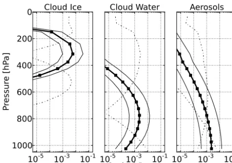
The overall design of the optimal estimation (OE) retrieval is described in O’Dell et al. (2012), Crisp et al. (2012) and Crisp et al. (2010). For this study, the B3.4 version of the al-gorithm is used, which has significant differences compared to the B2.9 algorithm documented in O’Dell et al. (2012). The newer algorithm retrieves two state variables related to fluorescence and uses a different aerosol parameterization. No fluorescence was included in the 3-D OCO2 simulator, so this part of the retrieval is disabled and the fluorescence vari-able values within the prior and first guess state vector are set to zero. In both the B2.9 and B3.4 versions, four atmospheric scatterers are used: water cloud, ice cloud, and “Kahn 2b” and “Kahn 3b” aerosols. The Kahn aerosol types are defined in Kahn et al. (2001). In the B3.4 version, the scattering parti-cles use a parameterized profile shape instead of allowing the profile to vary independently across pressure levels. For each of the four scatterer types, the profile is parameterized with a vertical Gaussian profile in optical depth, with three free parameters: the amplitude (the total optical depth), thickness, and height. The thickness and height are expressed in terms of pressure normalized by the surface pressure. The Gaus-sian profile is truncated when the vertical offset is near or below the surface, in which case the profile is renormalized such that the integral is equal to the total optical depth. Fig-ure 2 shows the prior profiles used in the retrieval along with the 1−σ perturbations to the total optical depth and height from the a priori covariance. The assumed prior values and variances are listed in Table 1. All covariances are assumed

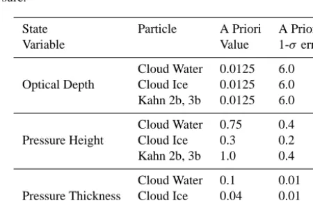
Table 1. A priori values and SDs for aerosol and cloud profiles. Note that the state vector contains the logarithm of the optical depth, so theσ range is a multiplicative scaling. The pressure heights and thicknesses are expressed as unitless ratios with the surface pres-sure.

State Particle A Priori A Priori Variable Value 1-σ error

Cloud Water 0.0125 6.0 Optical Depth Cloud Ice 0.0125 6.0 Kahn 2b, 3b 0.0125 6.0

Cloud Water 0.75 0.4 Pressure Height Cloud Ice 0.3 0.2 Kahn 2b, 3b 1.0 0.4

Cloud Water 0.1 0.01 Pressure Thickness Cloud Ice 0.04 0.01 Kahn 2b, 3b 0.2 0.01

to be zero. Note that the thickness is tightly constrained by the prior variance and is effectively a fixed parameter. This parameterization results in a maximum number of degrees of freedom of 8 for the scattering particles.

3.2 Pre-screening algorithm

Figure 2. Prior optical depth profiles. The thick solid line with square markers shows the per-layer optical depth prior profile; the solid lines show the±σrange applied to the optical depths; the dot-dashed lines show the±σrange applied to the pressure heights.

standard workstation at the University of Wisconsin (AMD OpteronTM 4180 CPU), this simplified model takes on the order of 30 s to compute one iteration of the OE algorithm (e.g., computing the forward model result and Jacobians at the state vector update). Compared to the data collection rate (24 observations per second), this implies that only a small fraction of the observations will be processed with the phys-ical OE retrieval. The target for initial operating capability is to apply the physical retrieval to 6 % of the total observa-tions. Thus, careful prescreening methods must be applied to the observations to select the subset most likely to produce accurateXCO2 retrievals. The precise form of the screening

method is itself a subject of research within the ACOS effort (Mandrake et al., 2013). In this study, the focus will be on the “A-band preprocessor” (ABP), described in Taylor et al. (2012). This prescreening algorithm uses a highly simplified, single-step retrieval of surface pressure and surface albedo, assuming a clear sky profile with only Rayleigh scattering. It uses a subset of the full A-band spectrum. Tests with this al-gorithm showed that the difference between the retrieved sur-face pressure and the interpolated ECMWF analysis sursur-face pressure is an effective cloud screen. The pressure difference is especially sensitive to higher altitude clouds that intro-duce large photon path modification. Observations that yield retrieved surface pressures much different than the forecast value (>±10 hPa) indicate significant cloud and/or aerosol contamination in the observed radiance (O’Dell et al., 2012). In effect, a thick cloud layer can act as a surface, so that the retrieved surface pressure is related to the cloud top pressure (CTP). This approach has been proposed as a retrieved cloud product for previous missions (for example, a CTP measure-ment for the O2 A-band was originally planned for Cloud-Sat, see Miller and Stephens, 2001). For OCO-2, however, the retrieved surface pressure will be primarily used to

re-move cloud-contaminated observations via the ABP. At this time is not possible to retrieveXCO2to the required accuracy

from the cloud-contaminated observations.

Following Taylor et al. (2012) and simulation tests with the B3.4 algorithm, a surface pressure threshold of 10 hPa is used for the ABP. In addition, aχ2 threshold is computed by the ABP, based on the noise level predicted by the sensor noise model (O’Dell et al., 2011) and the radiance level of the observation. If the computedχ2is larger than the threshold, the observation will be screened.

Cloud and aerosol contamination need not be directly in the sensor’s field of view, and may be produced by signif-icant multiple scattered radiation from clouds near the field of view. Such scattered radiation could cause either threshold (surface pressure orχ2) to be exceeded. In this more gen-eral sense, the ABP could be viewed as detecting “photon path modification” in the radiance observation, and thus the 1-D retrieval algorithm will not produce an accurateXCO2

retrieval.

3.3 Post-screening algorithm

In cases where the prescreening method does not correctly detect a cloud or aerosol contaminated spectrum, the retrieval may converge to an inaccurateXCO2 result. Therefore,

addi-tional post-screening is performed on the retrieved state vec-tor in an attempt to eliminate poor quality retrievals. These post screens are generally made by performing threshold tests on the retrieved surface pressure, surface albedos, re-trieved aerosol or cloud optical depths, and reducedχ2 val-ues for each band. The reducedχ2is the calculatedχ2value divided by the number of degrees of freedom, which is ex-pected to be close to 1 if the modeled and measured spectra differ only by random sensor noise. The first two post screen threshold tests are very similar to those used by the ABP, but use tighter threshold values. The latter two thresholds are motivated from simulation tests (O’Dell et al., 2012).

The values of the various post screening thresholds are continually adjusted for the ACOS products by analysis and comparisons of GOSAT and TCCON retrievals, in order to minimize the bias in the final retrievedXCO2. Thus the

partic-ular values prescribed in the B3.4 release documentation are not necessarily relevant to these simulation experiments, es-pecially for the reducedχ2thresholds for the spectral resid-uals. The residuals will include various model deficiencies (such as inaccurate absorption line spectroscopy) when com-pared with real data. No such effects are included in this sim-ulation and retrieval framework, so the reduced χ2 values will be close to the theoretical values. To deriveχ2 thresh-olds for these tests, an ensemble of simulated clear sky spec-tra (with aerosols but no cloud liquid water) was processed with the L2 algorithm. A threshold of 1.25 was selected for all three bands, which is 3.6 SDs above the mean reduced

Screening thresholds on the retrieved scattering optical depths are also important for high accuracy retrievals. The values used in B3.4 applied to GOSAT high-gain observa-tions over land are 0.15 for the sum of all four scatterers (cloud water, cloud ice, and both Kahn aerosol types), 0.07 for cloud water, and 0.045 for cloud ice. For the GOSAT medium-gain observations over land, these thresholds are 0.1, 0.07, and 0.03, for the total, cloud water, and cloud ice optical depths, respectively. Since these thresholds were em-pirically determined for the GOSAT data as processed with the B3.4 algorithm, they are not necessarily the best choice for this analysis. Tests with the clear sky retrievals show that these thresholds were somewhat too restrictive, and the se-lected thresholds in this analysis are 0.175, 0.1, and 0.03 for the total, cloud water, and cloud ice optical depths, respec-tively. These threshold values are consistent with the values selected for simulation-based tests (O’Dell et al., 2012), and are still more restrictive than the initially reported threshold of 0.3 in aerosol optical depth for performingXCO2retrievals

(Crisp et al., 2004).

4 Retrieval test setup

The specific tests are designed to explore potential retrieval biases caused by low level clouds. Even without considering 3-D scattering effects, low level layer clouds can be chal-lenging to identify (O’Dell et al., 2012). A low level layer cloud can introduce both photon path shortening and length-ening (Bennartz and Preusker, 2006), which can tend to can-cel and mask the cloud’s effect on the radiance measurement. The work presented here can be viewed as an extension of these previous 1-D simulation efforts to broken or isolated low clouds, which have strong 3-D scattering effects.

4.1 Scenarios

A single spheroidal liquid water cloud was created in the cen-ter of a 3.5 km (horizontal)×2.5 km (vertical) domain. The grid spacing is 100 m in all three dimensions. Dust aerosol is evenly distributed within the domain, with a total aerosol optical depth (AOD) of 0.05 in the vertical dimension. The cloud has an altitude of 1.6 km, and a fixed thickness of 0.6 km in the zaxis. Three cloud sizes are simulated, with the cloud diameter in the horizontal axes set to 0.6, 0.8 and 1.2 km. Therefore the smallest cloud is spherical, while the 0.8 and 1.2 km clouds are oblate spheroids. The liquid water con-tent (LWC) has a quadratic profile in all three dimensions. The cloud fraction within the blurred SRF (see Sect. 2.1) is not well defined, but it covers roughly 10, 20, and 40 % of the unblurred, rectangular nadir FOV for the three cloud sizes. The maximum LWC, in the center of the cloud, is 0.125 g m−3, yielding a maximum liquid water path (LWP) through the cloud center of 50 g m−2. The maximum visible optical depth along this same path is approximately 8. Two

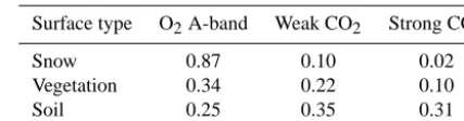
Table 2. Lambertian surface albedos, in each of the three OCO-2 spectral bands, for the three surface types.

Surface type O₂A-band Weak CO₂ Strong CO₂

Snow 0.87 0.10 0.02

Vegetation 0.34 0.22 0.10

Soil 0.25 0.35 0.31

solar zenith angles (SZAs) are used: 35, and 60◦. The surface is assumed to be Lambertian, with realistic albedo values in regions classified as snow, vegetated, and soil. Table 2 lists the selected values.

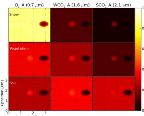
The SHDOM has the option to run with open or peri-odic boundary conditions. The periperi-odic boundary condition is used for all cases. SHDOM is used to simulated a nadir view using these LWC and aerosol fields. The cloud field is then a grid of identical clouds with a 3.5 km horizontal spacing, rather than a single isolated cloud. In Fig. 3, the nadir sensor view is shown for the three selected surface albe-dos for a single OCO-2 spectral channel in each of the three bands. The single channel is chosen at a wavelength between absorption lines so there is little extinction of the solar radia-tion. The views are shown for the 35◦solar zenith angle. 4.2 Creating OCO-2 spectra

Using the spectral data array described in Sect. 2.3, a syn-thetic OCO-2 observation is generated by applying the surro-gate SRF (see Sect. 2.1). The 2-D nadir radiance array at each channel frequency is multiplied by the SRF and summed to produce the OCO-2 channel radiance. Figure 4 shows ex-amples of the SRF applied to a low absorption O2A band channel. The SRF is applied at various positions, by scan-ning left-to-right over the cloud in the scene. A total of 25 SRF centered positions are used, where the SRF is shifted by a single 100 m grid cell, and the 10th position is centered in the 3.5 km domain. Positions 0, 5, 10, 15 and 20 (i.e., the center of the SRF falls at positions 0.75, 1.25, 1.75, 2.25 and 2.75 km along thex axis in the 100 m grid) are shown in Fig. 4. The SRF positions move between regions dominated by clear, cloudy or shadowed high resolution grid cells, de-pending on the cloud size and solar zenith angle. For brevity, the positions will be referred to as clear, cloudy and shadow, depending on which type of high resolution pixel is domi-nant at that location, but it is apparent that in all cases the SRF will contain a mixture of all three types.

Figure 3. Overhead views of the scene reflectance as simulated by SHDOM, for a channel within each OCO-2 band that has relatively low gas absorption. Each of the three columns shows the reflectance for one of the three OCO-2 bands, and each of the three rows shows reflectance from one surface type. All images are shown with the same display scale, to highlight the differences in contrast between the cloud and surface for the different spectral bands and surface types.

are processed with the ABP algorithm and the B3.4 L2 re-trieval code, and the relevant quantities are averaged over the ensemble members. The ABP uses a subset of the O2A band (759.18–760.75 nm), while the L2 retrieval runs on the full 3-band spectra. The L2 retrieval uses an input meteorology data set (in operations, this is taken from a numerical weather forecast), which is set to the truth values. In other words, the meteorology sent to the L2 retrieval is the same meteorol-ogy data used to simulate the spectra with the 3-D OCO-2 simulator.

5 Retrieval test results 5.1 Screening rates

In normal operations, the results of the ABP would be ap-plied before performing L2 retrievals. In cases where 3-D effects are important, it is possible that the ABP could pref-erentially identify cloudy observations in cases where the full L2 algorithm can produce accurate retrievals. This behavior would not have been captured in the development of the ABP, since all radiative transfer models used in the earlier studies were plane parallel. Therefore, in these experiments, the L2 algorithm is applied to all simulated observations, regardless of the output from the ABP. This allows full characteriza-tion of the ABP performance, to verify that it is removing the cloud-contaminated observations that the L2 algorithm cannot accurately process.

5.1.1 ABP prescreening

Recall that at each SRF position, an ensemble of 37 spectra were generated with independent sensor noise. The ensem-ble allows for a screening fraction to be computed at each position. Figure 5 shows these fractions as a function of SRF position, for the various scenarios. The ABP’s performance appears directly correlated to the O2A band albedo and the cloud size, as expected. Recall that the ABP retrieves just the surface pressure from the O2A band (see Sect. 3). Over snow, since the surface is much more reflective, a larger proportion of the observed radiance is due to the single scattering off the surface, which will tend to pull the retrieved pressure to the surface value. The ABP also detects a cloud mainly when the SRF is centered on the cloud, but not in the primarily “clear” or “shadow” positions. A single screening rate for each sce-nario can be computed by averaging over the SRF positions. Table 3 shows these results.

5.1.2 Postscreener

Figure 6 shows the postscreening fractions, with the same layout as Fig. 5 showing the prescreening fractions. The postscreening fractions are defined with respect to the total number of simulated observations, since the L2 retrieval was run on all observations, not just the ones that were not identi-fied as cloudy by the ABP. Ideally, the postscreened fractions should be equal or higher than the prescreened fractions from the ABP. This would imply that the ABP correctly identified an observation that would not have produced an accurate L2 retrieval. A higher postscreening fraction is also expected, since the L2 retrieval has access to more information (since it retrieves from all 3 OCO-2 bands), and uses a more com-plicated state vector.

For the vegetation and soil surfaces with 60◦solar zenith angle, the postscreening fractions as a function of the SRF position are extremely similar to the prescreening fractions. For the remaining cases, except for the soil surface at 35◦ solar zenith angle, the post screening method tends to iden-tify a much larger fraction of cloudy observations. This is especially true over snow where the fraction reaches nearly 100 % for the 0.8 km cloud. The outlier scenario here is the soil surface at 35◦solar zenith angle, where the ABP iden-tifies a much higher rate of cloud contamination than the postscreener. This behavior could be described in two ways: either the ABP could be improperly identifying these obser-vations, (if these retrievals produce accurateXCO2retrievals)

or the postscreener could be failing (if the retrievedXCO2 is

not accurate). This behavior will be discussed below in the context of the state variable biases.

Table 3. Percentage of simulated observations identified as cloudy by prescreener algorithm.

Surface Cloud Prescreen Pct. Prescreen Pct. Type Size SZA=35◦ SZA=60◦

Snow clear 0.0 0.0

Snow 0.6 km 0.0 0.0 Snow 0.8 km 0.0 0.0

Snow 1.2 km 0.0

Vege clear 0.0 0.0

Vege 0.6 km 0.0 0.0 Vege 0.8 km 0.0 0.0

Vege 1.2 km 40.2

Soil clear 0.0 0.0

Soil 0.6 km 0.0 0.0 Soil 0.8 km 34.6 11.6

Soil 1.2 km 70.3

that the postscreen could be improved with scene dependent thresholds.

5.2 State variable bias

In order to quantify the impact of 3-D radiative transfer ef-fects on the retrieved state variables, the retrieval outputs will be compared both to the known truth values as well as the re-sults from the cloud-free simulations. Since the ACOSXCO2

retrieval is known to have biases even for clear sky retrievals (O’Dell et al., 2012; Wunch et al., 2011b), the cloud-free simulations help to separate the bias caused by 3-D radia-tive transfer effects from the clear sky bias already present in the retrieval. In any particular scenario, the bias due to 3-D effects will be the difference between the bias computed in the cloudy retrievals and the bias computed in the clear sky retrievals.

As an initial example, the previous case noted in the screening discussion above is revisited. For the 0.8 km cloud, over the soil surface with solar zenith of 35◦, the ABP iden-tified all spectra with the SRF centered above the cloud as cloud contaminated. However, the postscreen only found about 20 % of these observations to be cloud contaminated. Figure 7 shows the bias in the retrievedXCO2 as a function

of the SRF position for this scenario. The bias is defined as the retrieved values, minus the known truthXCO2 value. The

left subplot shows all converged retrievals; the middle plot shows the screened retrievals (both prescreen and postscreen are applied). The set of retrievals shown in the middle plot would be the actual set retrieved by the full end-to-end L2 processing algorithm. The gap in observations around SRF position 10 is due to the ABP. The solid horizontal line shows the mean retrieved XCO2 from the clear sky retrievals

per-formed for this scenario; the bold error bar marker centered on zero bias shows the 1−σrange predicted by the posterior

covariance from the optimal estimation algorithm. Finally, to summarize the scatter plots, the distribution of points is con-densed down to a single box plot in the right subplot, and the number of points in each is marked along the bottom axis. The remaining bias distribution plots will match this layout, with the results condensed into the pair of box plots. The

XCO2 biases shown here indicate that the L2 retrieval is able

to compute an accurate valueXCO2 for all cases in this

sce-nario. This suggests that the ABP may be too aggressive in identifying cloud contamination in this scenario.

5.2.1 XCO2

Figure 8 contains theXCO2retrieval bias summary for all

sce-narios including the 0.6 and 0.8 km clouds. The 1.2 km cloud scenarios are not included here, since the screening rates are high for these cases. The different surface albedos are orga-nized by row, with the snow, vegetated and soil surfaces in the top, middle, and bottom rows, respectively.

For the snow surface, theXCO2biases are large, especially

for the 60◦solar zenith angle. The 0.6 km cloud case shows a consistent−5 ppm bias, which is 4 ppm lower than the clear sky bias. In this case only 12.5 % of the observations would be screened. For the 0.8 km cloud case, the screening does reduce the bias magnitude, from−9 to−6 ppm. This is the only case where the screening algorithms substantially re-duce the bias magnitude. Over the vegetated surface, the ab-solute biases are much smaller. The mean biases are within 2 ppm of truth, and within 3 ppm of the clear sky value. Fi-nally, over soil, the biases are well represented by the clear sky values. All biases are within approximately 0.3 ppm of the clear sky bias.

Overall, the magnitude of the biases seem to be most strongly related to the SCO2 surface albedo. In practice, an additional postscreen filter on the retrieved SCO2 is used, which was not used in these tests. A simple cutoff of about 0.05 albedo in the SCO2 band would essentially remove all the snow observations. The results here suggest the retrievals over snow are the most sensitive to 3-D radiative transfer ef-fects, further supporting the use of a screening threshold in the SCO2 band.

5.2.2 Surface albedo

Figure 4. Overhead view of the scene reflectance multiplied by the SRF at positions 0, 5, 10, 15, and 20, for the 0.6 km cloud in the O2 A-band over the soil surface. The SRF moves from left to right over the high spatial resolution grid. The top row shows the SRF sequence for the 35◦solar zenith angle (SZA), and the bottom row shows the sequence for the 60◦SZA. In the top row, the SRF starts at a position where the FOV is primarily filled with a “clear” surface view, to a “cloudy” position, and ends at a “shadowed” position. In the bottom row, the periodic boundary condition used in SHDOM causes the shadow to wrap around to the other side of the high spatial resolution scene for the larger SZA. For this case, the SRF starts in the “shadowed” position, followed by “cloudy” and then “clear”.

Figure 5. Fraction of simulated spectra identified as cloudy by the prescreening algorithm.

position 10 (the position centered on the cloud), which is also where the retrieved SCO2 albedo is the most accurate. The result is that the bias range, shown by the box plot, is not reduced.

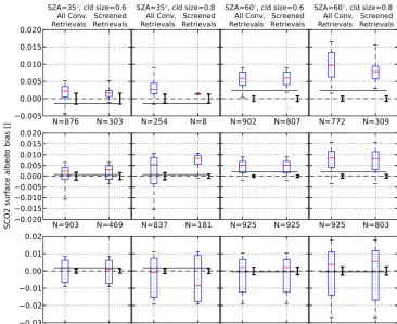
The summary of SCO2 albedo biases is shown in Fig. 10. Although the albedo bias is within the range 0.01–0.02 in all cases, the bias relative to the SCO2 albedo is substan-tial. A 0.01 albedo bias relative to the 0.02, 0.10, and 0.31 albedo values, for the snow, vegetated, and soil surfaces, re-spectively, is a relative bias of approximately 50, 10 and 3 %.

Figure 6. Fraction of simulated spectra identified as cloudy by the post screening algorithm.

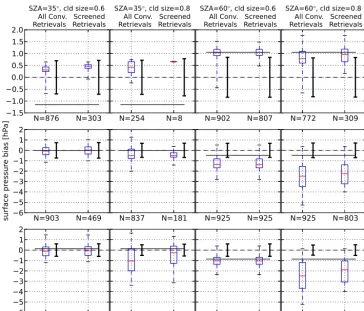
5.2.3 Surface pressure

The final retrieved variable for CO2concentration is the dry air mole fraction (theXCO2), which is equivalent to the ratio

of CO2molecules and O2molecules in the column. The lat-ter value is represented by the surface pressure, since the O2 concentration varies much less than the CO2concentration. This implies that any bias in the retrieved surface pressure will directly cause bias in the retrievedXCO2. Plots for

Figure 7. Bias in retrieved XCO2, showing the scatter plot of all

retrievals (left panel) and screened retrievals (middle panel), com-pared to the single box plot summarizing the bias (right panel). The error bar drawn with a thick black line, centered on zero bias, is the predicted posterior error (1σ) from the optimal estimation al-gorithm. The thin horizontal line marks the mean bias for retrievals from a cloud-free simulation. Finally, the number of retrievals in each box plot is indicated at the bottom of thexaxis in the right panel.

the bias plots in the previous sections forXCO2 and SCO2

surface albedo.

Since surface pressure is used in the ABP and for postscreening, large surface pressure bias will cause the ob-servation to be screened. In Fig. 11, the maximum abso-lute surface pressure bias is in the cloud-centered SRF po-sitions. These are the most likely to be screened, so in this case the overall surface pressure bias is reduced somewhat by the screening algorithms. The summary plot, in Fig. 12, shows that the overall reduction in bias only occurs in a few scenarios (both SZA for cloud size 0.8 km over the soil sur-face). The general patterns in the surface pressure bias are different than those seen in XCO2. For XCO2, the soil

sur-face retrievals show bias very similar to the clear sky bias, and then the bias increased as the SCO2 albedo decreased, resulting in very large bias over the snow surface. The re-sults for surface pressure are more related to the O2A albedo, since most of the sensitivity to surface pressure comes from the O2A band measurement. Thus, the surface pressure bias for the retrievals over the snow surface is quite different than the vegetation and soil surface albedos. The absolute bias for the retrievals over the snow surface albedo is about 1.5 hPa for the 35◦_{SZA and less than 0.3 hPa for the 60}◦_{SZA. The}

bias for the retrievals over the vegetation and soil surfaces are similar, with nearly zero bias for the 0.6 km cloud and 35◦ SZA, and larger absolute bias for the larger cloud size and SZA.

5.2.4 XCO2 and surface pressure

Since the XCO2 is directly related to the surface pressure,

the joint distribution of bias between these two variables is worth examining. Figure 13 shows scatter plots of the bi-ases for these two variables. Each panel corresponds to a

sin-Table 4. Percentage of simulated observations identified as cloudy by postscreener algorithm.

Surface Cloud Postscreen Pct. Postscreen Pct. Type Size SZA=35◦ SZA=60◦

Snow clear 28.4 1.4

Snow 0.6 km 67.0 12.5 Snow 0.8 km 98.1 66.6

Snow 1.2 km 95.8

Vege clear 1.4 0.0

Vege 0.6 km 48.2 0.0 Vege 0.8 km 80.0 13.2

Vege 1.2 km 68.8

soil clear 2.7 0.0

soil 0.6 km 12.5 0.0 soil 0.8 km 32.3 13.2

soil 1.2 km 71.7

gle scenario, matching the layout seen earlier in Fig. 8. The black points show the biases for the individual screened re-trievals, and the large cyan cross shows the clear sky retrieval bias. The overplotted ellipse in the lower left corner is an ex-ample posterior covariance from the optimal estimation al-gorithm. The covariance is computed for each retrieval, but within each scenario the covariance does not change signifi-cantly between each retrieval. Note that the display scales in both thexandyaxes are different in each row of plot panels (corresponding to a single surface albedo). The “flattened” appearance of the covariance ellipses for the snow surface albedo scenarios is largely due to the largey-range for the

XCO2 bias display. The ellipse orientation describes the

de-gree of covariance between the two variables, as calculated by the optimal estimation algorithm. It is clear that there is no consistent strong covariance, but rather a weak covariance that is scenario dependent. The retrieval biases also show cor-relation that is dependent on the scenario. The corcor-relation is highest in the 60◦SZA, vegetation scenario, and very low in all scenarios using the soil albedo.

5.2.5 Profiles of atmospheric scatterers

Figure 8. Summary ofX_CO2 retrieval bias for all scenarios with 0.6 and 0.8 km clouds. See Fig. 7 for details.

Figure 9. Bias in retrieved SCO2 albedo, with the same layout as Fig. 7.

surface are shown. Note that the retrieval estimates a signifi-cant amount of cloud ice optical depth at high altitudes, even though the simulation did not include any cloud ice at any level, and no scatterers above the 700 hPa level other than molecular scattering. The gap in the middle of the second column (the 0.8 km cloud size, and 35◦SZA) is due to the complete screening of these retrievals.

6 Discussion

The overall purpose of the prescreening algorithm is to quickly identify observations that are sufficiently contami-nated by cloud to preclude accurate Level 2XCO2retrievals.

Characterizing its performance for the scenarios here must involve a discussion of the prescreening rate as well as the

XCO2 bias with and without applying the prescreening.

In general, the ABP cannot detect the smallest sub-FOV cloud (0.6 km diameter), and has limited ability to detect the larger clouds (0.8 and 1.2 km diameter). It is important to note however that the reasonable accuracy of the ABP algorithm in identifying homogeneous cloudy scenes, i.e, 100 % FOV contamination, has been shown on simulated data (O’Dell et al., 2012). Furthermore, comparisons were favorable against the MODIS cloud mask for select GOSAT soundings (Taylor et al., 2012). The screening fraction is re-lated to the albedo in the O2A band, as the screening rates are highest for the soil surface, and zero for the snow surface (see Table 3 and Fig. 5). Likely this is due to poor contrast between the surface and cloud when the surface is bright (for example, in Fig. 3 the cloud is barely discernible over the snow surface in the O2A band). For the snow surface, the

XCO2 biases are often quite large, up to 5–10 ppm, so the

Screen-1652 A. Merrelli et al.: Bias in OCO-2 retrievals caused by 3-D radiation scattering −0.005 0.000 0.005 0.010 0.015 0.020 N=876 N=303 SZA=35°, cld size=0.6 All Conv. Screened Retrievals Retrievals

N=254 N=8 SZA=35°, cld size=0.8 All Conv. Screened Retrievals Retrievals

N=902 N=807 SZA=60°, cld size=0.6 All Conv. Screened Retrievals Retrievals

N=772 N=309 SZA=60°, cld size=0.8 All Conv. Screened Retrievals Retrievals

−0.020 −0.015 −0.010 −0.005 0.000 0.005 0.010 0.015 0.020 SC O 2 su rf ac e al be do b ia s []

N=903 N=469 N=837 N=181 N=925 N=925 N=925 N=803

−0.03 −0.02 −0.01 0.00 0.01 0.02

N=925 N=809 N=921 N=377 N=925 N=925 N=925 N=735

A lb ed o = sn ow A lb ed o = v eg e A lb ed o = so il

Figure 10.

Summary of SCO2 surface albedo retrieval bias for all

scenarios with 0.6 and 0.8

km

clouds, with the same layout as Fig. 8.

0 5 10 15 20 25

SRF Position

0 5 10 15 20 25

SRF Position

Screened Retrievals

N=921 N=377

SZA=35°, cloud size=0.8 All Converged Screened

Retrievals Retrievals

A lb ed o = so il

Figure 11.

Bias in retrieved surface pressure, with the same layout

as Fig. 7.

−1.5 −1.0 −0.5 0.0 0.5 1.0 1.5 2.0 N=876 N=303 SZA=35°, cld size=0.6 All Conv. Screened Retrievals Retrievals

N=254 N=8 SZA=35°, cld size=0.8 All Conv. Screened Retrievals Retrievals

N=902 N=807 SZA=60°, cld size=0.6 All Conv. Screened Retrievals Retrievals

N=772 N=309 SZA=60°, cld size=0.8 All Conv. Screened Retrievals Retrievals

−6 −5 −4 −3 −2 −1 0 1 2 su rf ac e pr essu re b ia s [h Pa ]

N=903 N=469 N=837 N=181 N=925 N=925 N=925 N=803

−6 −5 −4 −3 −2 −1 0 1 2

N=925 N=809 N=921 N=377 N=925 N=925 N=925 N=735

A lb ed o = sn ow A lb ed o = v eg e A lb ed o = so il

Figure 12.

Summary of surface pressure retrieval bias for all

sce-Figure 13.

Summary of surface pressure and

X

CO

retrieval bias

and covariance for all scenarios with 0.6 and 0.8

km

clouds. Plot

panels are arranged in the same order as Fig. 8. In each panel, the

screened retrievals are shown (black points) along with the mean

clear sky retrieval (large cyan cross). The ellipse shows the

1

σ

pos-terior covariance for these two retrieved variables, offset by an

ar-bitrary amount for display clarity.

Figure 14.

Retrieved optical depth profiles of atmospheric

scatter-ers for four scenarios (cloud sizes 0.6 and 0.8

km

for both SZA)

with the soil surface albedo. Each panel shows the profile in a

ver-tical column, with the

y

axis indicating profile pressure, and the

x

axis indicating the SRF position. Top, middle and bottom rows

show the cloud water, cloud ice, and aerosol (sum of the Khan 2b

and 3b) profiles, respectively. The far right column shows the prior

optical depth profiles used by the optimal estimation retrieval.

Figure 10. Summary of SCO2 surface albedo retrieval bias for all scenarios with 0.6 and 0.8 km clouds, with the same layout as Fig. 8.

Figure 11. Bias in retrieved surface pressure, with the same layout as Fig. 7.

ing out retrievals over snow surfaces could easily be achieved by other simple tests. For example, filtering could be done seasonally by latitude to exclude retrievals over likely snow covered regions, or by requiring a minimum signal level in the SCO2 band. Operationally, the ACOS retrieval algorithm has taken similar steps to avoid retrievals over snow and ice surfaces, by using thresholds on the retrieved albedos to ex-clude likely snow or ice covered surfaces. These thresholds remove retrievals with very low SCO2 albedo, or retrievals with a combination of very high O2A albedo and low SCO2 albedo. Over the vegetated surface, the biases are smaller,

but still significant, up to 2 ppm to the known truth value and up to 3 ppm relative to the clear sky bias value. These scenarios are the most concerning for the ABP. The soil sur-face, in contrast, yields very accurateXCO2 retrievals, with

bias less than 1.5 ppm relative to the known truth value and within 0.3 ppm relative to the clear sky bias value. In fact, the L2 retrieval yields accurateXCO2 retrievals even for the

pre-screened observations, indicating the ABP is too restrictive in some cases.

The postscreen filters applied after the L2 retrieval are much more effective at identifying the cloud contamination. In nearly all surface and SZA scenarios the 0.8 km cloud is identified in more than half of the observations. The vege-tated and soil surfaces for 60◦solar zenith angle are the ex-ception, but the majority of cases are screened at the 1.2 km cloud size.

TheXCO2 biases on the final screened retrievals are

gen-erally equivalent to the bias from the set of all converged re-trievals. This is illustrated with the box plots in Fig. 8. If the screening methods were preferentially identifying highXCO2

bias retrievals, then the box plot for the screened retrieval set should be narrower and closer to the clear sky bias. However, in all cases the two box plots are equivalent.

For other retrieved state variables, the bias is more signif-icant. The SCO2 albedo bias results shown in Figs. 9 and 10 show similar behaviors as theXCO2bias. Specifically, the

Figure 12. Summary of surface pressure retrieval bias for all scenarios with 0.6 and 0.8 km clouds, with the same layout as Fig. 8.

bias is largest for snow, and smallest for soil, and the screen-ing does not reduce the mean absolute bias. The latter ef-fect can be clearly seen in Fig. 9, since the screening tends to remove observations at SRF position 10 (centered on the cloud), where the retrieved SCO2 albedo is close to the truth value.

The retrieved optical depth profiles for the scattering par-ticles also exhibit large biases. Figure 14 shows the results for four soil surface cases (0.6 and 0.8 km clouds at both so-lar zenith angles). The profiles show complicated relation-ships to the SRF positions, with both the total optical depths and the profile altitudes changing as the SRF scans over the scene. Note that from the screening rate results (Tables 3 and 4) most of these retrievals are passed by both screen-ing algorithms. Since the reducedχ2was used as part of the postscreen algorithm, the spectral residuals are small. Thus the 1-D radiative transfer model is able to recreate the spectra simulated with the 3-D radiative transfer code well enough to produce lowχ2values and pass the screening algorithm. Thus the patterns in the optical depth profiles represent dif-ferent 1-D plane parallel representations of the 3-D scattering field in the simulations. These scatterer profiles are very dif-ferent from the true 3-D distributions. Recall from Sect. 4 that the aerosol layer in the model is evenly distributed in the lower 2.5 km, which is the approximately the pressure layer

for P >700 hPa, while the cloud is located at an altitude of 1.6 km (approximately 800 hPa). The retrieved scatterer profiles are displaced vertically as the SRF position moves across the cloud, but the actual scatterers are at fixed alti-tudes. Only the results for the retrievals over the soil surface are shown here. The retrievals over other surfaces show qual-itatively similar behavior, in that the scatterer vertical profiles change significantly with the SRF position.

7 Conclusions

By processing simulated OCO-2 observations created with a 3-D radiative transfer model, the impact of 3-D scatter-ing effects has been estimated for the scenario of low alti-tude, sub-FOV liquid water clouds. Tests were done for two solar zenith angles (35 and 60◦_{), and three surface types}

(snow, vegetation, and soil). Overall, the retrieved XCO2

shows biases that are strongly dependent on the SCO2 sur-face albedo. After screening, the worst case mean bias over snow is roughly 5 ppm relative to clear sky retrievals, for the 0.8 km cloud and 60◦ solar zenith angle. At the other ex-treme, the mean retrieved XCO2 bias is less than 0.5 ppm

Figure 13. Summary of surface pressure andXCO2retrieval bias and covariance for all scenarios with 0.6 and 0.8 km clouds. Plot panels are

arranged in the same order as Fig. 8. In each panel, the screened retrievals are shown (black points) along with the mean clear sky retrieval (large cyan cross). The ellipse shows the 1σ posterior covariance for these two retrieved variables, offset by an arbitrary amount for display clarity.

ABP has difficulty identifying these sub-FOV clouds, but in many cases the L2 retrieval is still able to retrieve an accu-rateXCO2. Neither screening method reduces the mean bias

within a single test case. From the overall perspective of the entire group of tests, the screening methods do reduce bias by screening higher fractions of the larger clouds sizes which do have largerXCO2 bias. Both screening methods

primar-ily detect the cloud-centered SRF positions, so the shadow-contaminated observations are detected less often.

While the analysis presented here does indicate potentially large biases in the OCO-2XCO2 retrievals, at present we do

not know the potential impact on the global XCO2 data set.

A future study is needed to connect these results to measured spatial and temporal distribution of clouds. The resulting bias in a global XCO2 data set will depend on the occurrence of

cloudy scenes similar to the presented synthetic scenarios. The biases could be especially problematic if they are re-gionally correlated.

During this study, development has continued on the oper-ational retrieval algorithm past version B3.4. The treatment of aerosols is quite different in more recent versions. A ge-ographically dependent aerosol climatology is used to select the pair of aerosols used for each retrieval from a set of six aerosol types. Clearly the retrieval biases among the albedo and aerosol profiles are highly correlated, so the quantitative behavior may be very different in the new algorithm. How-ever the general behavior of the retrieved aerosol profile – where it is highly dependent on the unresolved 3-D cloud field – should remain unchanged.

Finally, one important caveat on these results is the re-liance on an unpolarized forward model. Since the actual OCO-2 measurement is polarized, these results should be re-peated with the same framework using a fully polarized 3-D radiative transfer model. It is unknown how the retrieval will behave differently when working with the(I−Q)/2 radiance instead of the unpolarized radiance. In addition, it would be important to extend these analyses to the glint mode obser-vation. Polarized radiative transfer is even more important for simulating glint mode observation, since the glint mode relies on the strongly polarized specular reflection from the ocean surface. Since this project began, the SHDOM model has been improved and now can perform the polarized radia-tive transfer (Evans, 2014).

Acknowledgements. This research project was supported by the NASA OCO-2 Science Team, under contract NNX13AB97G. The authors thank the Space Science and Engineering Center Technical Computing group for providing cluster computing resources used for the simulations.

Edited by: H. Worden

References

Bennartz, R. and Preusker, R.: Representation of the photon path-length distribution in a cloudy atmosphere using finite ele-ments, J. Quant. Spectrosc. Ra., 98, 202–219, 2006.

Bovensmann, H., Buchwitz, M., Burrows, J. P., Reuter, M., Krings, T., Gerilowski, K., Schneising, O., Heymann, J., Tret-ner, A., and Erzinger, J.: A remote sensing technique for global monitoring of power plant CO₂emissions from space and related applications, Atmos. Meas. Tech., 3, 781–811, doi:10.5194/amt-3-781-2010, 2010.

Buchwitz, M., Schneising, O., Burrows, J. P., Bovensmann, H., Reuter, M., and Notholt, J.: First direct observation of the at-mospheric CO2year-to-year increase from space, Atmos. Chem. Phys., 7, 4249–4256, doi:10.5194/acp-7-4249-2007, 2007. Crisp, D. and Johnson, C.: The Orbiting Carbon

Ob-servatory mission, Acta Astronaut., 56, 193–197, doi:10.1016/j.actaastro.2004.09.032, 2005.

Crisp, D., Atlas, R., Breon, F.-M., Brown, L., Burrows, J., Ciais, P., Connor, B., Doney, S., Fung, I., Jacob, D., Miller, C., O’Brien, D., Pawson, S., Randerson, J., Rayner, P., Salaw-itch, R., Sander, S., Sen, B., Stephens, G., Tans, P., Toon, G., Wennberg, P., Wofsy, S., Yung, Y., Kuang, Z., Chudasama, B., Sprague, G., Weiss, B., Pollock, R., Kenyon, D., and Schroll, S.: The Orbiting Carbon Observatory (OCO) mission, Adv. Space Res., 34, 700–709, 2004.

Crisp, D., Bösch, H., Brown, L., Castano, R., Christi, M., Con-nor, B., Frankenberg, C., McDuffie, J., Miller, C. E., Natraj, V., O’Dell, C., O’Brien, D., Polonsky, I., Oyafuso, F., Thompson, D., Toon, G., and Spurr, R.: OCO (Orbiting Carbon Observatory)-2 Level Observatory)-2 Full Physics Retrieval Algorithm Theoretical Basis, 2010.

Crisp, D., Fisher, B. M., O’Dell, C., Frankenberg, C., Basilio, R., Bösch, H., Brown, L. R., Castano, R., Con-nor, B., Deutscher, N. M., Eldering, A., Griffith, D., Gunson, M., Kuze, A., Mandrake, L., McDuffie, J., Messerschmidt, J., Miller, C. E., Morino, I., Natraj, V., Notholt, J., O’Brien, D. M., Oyafuso, F., Polonsky, I., Robinson, J., Salawitch, R., Sher-lock, V., Smyth, M., Suto, H., Taylor, T. E., Thompson, D. R., Wennberg, P. O., Wunch, D., and Yung, Y. L.: The ACOS CO2 retrieval algorithm – Part II: GlobalXCO2 data characterization,

Atmos. Meas. Tech., 5, 687–707, doi:10.5194/amt-5-687-2012, 2012.

Dubovik, O., Holben, B., Eck, T. F., Smirnov, A., Kaufman, Y. J., King, M. D., Tanré, D., and Slutsker, I.: Variability of absorption and optical properties of key aerosol types observed in world-wide locations, J. Atmos. Sci., 59, 590–608, 2002.

Evans, K. F.: The spherical harmonics discrete ordinate method for three-dimensional atmospheric radiative transfer, J. Atmos. Sci., 55, 429–446, 1998.

Evans, K. F.: Polarized SHDOM, American Meteorological So-ciety, 14th Conference on Atmospheric Radiation, Boston, MA, July 2014, available at: https://ams.confex.com/ams/ 14CLOUD14ATRAD/webprogram/Paper249476.html (last ac-cess: 20 November 2014), 2014.

Kahn, R., Banerjee, P., and McDonald, D.: Sensitivity of multiangle imaging to natural mixtures of aerosols over ocean, J. Geophys. Res.-Atmos., 106, 18219–18238, 2001.

Mandrake, L., Frankenberg, C., O’Dell, C. W., Osterman, G., Wennberg, P., and Wunch, D.: Semi-autonomous sounding selection for OCO-2, Atmos. Meas. Tech., 6, 2851–2864, doi:10.5194/amt-6-2851-2013, 2013.

Miller, C. E., Crisp, D., DeCola, P. L., Olsen, S. C., Rander-son, J. T., Michalak, A. M., Alkhaled, A., Rayner, P., Ja-cob, D. J., Suntharalingam, P., Jones, D. B. A., Denning, A. S., Nicholls, M. E., Doney, S. C., Pawson, S., Boesch, H., Con-nor, B. J., Fung, I. Y., O’Brien, D., Salawitch, R. J., Sander, S. P., Sen, B., Tans, P., Toon, G. C., Wennberg, P. O., Wofsy, S. C., Yung, Y. L., and Law, R. M.: Precision requirements for space-based XCO2 data, J. Geophys. Res.-Atmos., 112, D10314,

doi:10.1029/2006JD007659, 2007.

Miller, S. D. and Stephens, G. L.: CloudSat instrument requirements as determined from ECMWF forecasts of global cloudiness, J. Geophys. Res.-Atmos., 106, 17713–17733, 2001.

O’Brien, D. M., Polonsky, I., O’Dell, C., and Carheden, A.: Orbit-ing Carbon Observatory (OCO), algorithm theoretical basis doc-ument: the OCO simulator, Technical report ISSN 0737-5352-85, Cooperative Institute for Research in the Atmosphere, Col-orado State University, 2009.

O’Dell, C., Day, J., Pollock, R., Bruegge, C., O’Brien, D., Cas-tano, R., Tkatcheva, I., Miller, C., and Crisp, D.: Preflight ra-diometric calibration of the orbiting carbon observatory, IEEE T. Geosci. Remote, 49, 2438–2447, 2011.

O’Dell, C. W., Connor, B., Bösch, H., O’Brien, D., Frankenberg, C., Castano, R., Christi, M., Eldering, D., Fisher, B., Gunson, M., McDuffie, J., Miller, C. E., Natraj, V., Oyafuso, F., Polon-sky, I., Smyth, M., Taylor, T., Toon, G. C., Wennberg, P. O., and Wunch, D.: The ACOS CO2 retrieval algorithm – Part 1: De-scription and validation against synthetic observations, Atmos. Meas. Tech., 5, 99–121, doi:10.5194/amt-5-99-2012, 2012. Taylor, T., O’Dell, C., O’Brien, D., Kikuchi, N., Yokota, T.,

Naka-jima, T., Ishida, H., Crisp, D., and NakaNaka-jima, T.: Comparison of cloud-screening methods applied to GOSAT near-infrared spec-tra, IEEE T. Geosci. Remote, 50, 295–309, 2012.

Thompson, D. R., Chris Benner, D., Brown, L. R., Crisp, D., Malathy Devi, V., Jiang, Y., Natraj, V., Oyafuso, F., Sung, K., Wunch, D., Castaño, R., and Miller, C. E.: Atmospheric valida-tion of high accuracy CO2absorption coefficients for the OCO-2 mission, J. Quant. Spectrosc. Ra., 113, 2265–2276, 2012. Tran, H. and Hartmann, J.-M.: An improved O2 A band

absorp-tion model and its consequences for retrievals of photon paths and surface pressures, J. Geophys. Res.-Atmos., 113, D18104, doi:10.1029/2008JD010011, 2008.

Várnai, T., Marshak, A., and Yang, W.: Multi-satellite aerosol obser-vations in the vicinity of clouds, Atmos. Chem. Phys., 13, 3899– 3908, doi:10.5194/acp-13-3899-2013, 2013.

Wunch, D., Toon, G. C., Blavier, J.-F. L., Washenfelder, R. A., Notholt, J., Connor, B. J., Griffith, D. W. T., Sherlock, V., and Wennberg, P. O.: The total carbon column observing network, Philos. T. R. Soc. A, 369, 2087–2112, 2011a.

Wunch, D., Wennberg, P. O., Toon, G. C., Connor, B. J., Fisher, B., Osterman, G. B., Frankenberg, C., Mandrake, L., O’Dell, C., Ahonen, P., Biraud, S. C., Castano, R., Cressie, N., Crisp, D., Deutscher, N. M., Eldering, A., Fisher, M. L., Griffith, D. W. T., Gunson, M., Heikkinen, P., Keppel-Aleks, G., Kyrö, E., Lin-denmaier, R., Macatangay, R., Mendonca, J., Messerschmidt, J., Miller, C. E., Morino, I., Notholt, J., Oyafuso, F. A., Ret-tinger, M., Robinson, J., Roehl, C. M., Salawitch, R. J., Sher-lock, V., Strong, K., Sussmann, R., Tanaka, T., Thompson, D. R., Uchino, O., Warneke, T., and Wofsy, S. C.: A method for eval-uating bias in global measurements of CO2total columns from space, Atmos. Chem. Phys., 11, 12317–12337, doi:10.5194/acp-11-12317-2011, 2011b.

Yoshida, Y., Ota, Y., Eguchi, N., Kikuchi, N., Nobuta, K., Tran, H., Morino, I., and Yokota, T.: Retrieval algorithm for CO2and CH4 column abundances from short-wavelength infrared spectral ob-servations by the Greenhouse gases observing satellite, Atmos. Meas. Tech., 4, 717–734, doi:10.5194/amt-4-717-2011, 2011. Zhang, Z., Ackerman, A. S., Feingold, G., Platnick, S., Pincus, R.,