DISOCIAL MEDIA SYNCHRONIZATION MODEL: IN ASSOCIATION WITH DEVELOPING SMALL MEDIUM ENTERPRISES SALES INFORMATION SYSTEM

401

A RELIABLE AND ENERGY EFFICIENT ROUTING

ALGORITHM IN WSN USING LEARNING AUTOMATA

1

RAZIEH ASGARNEZHAD, 2NASER NEMATBAKHSH

1_{Department of Computer Engineering, Isfahan (Khorasgan) Branch, Islamic Azad University, Isfahan, Iran}

2_{Faculty of Computer Engineering, Najafabad Branch, Isfahan Azad University, Najafabad, Isfahan, Iran}

E-mail: 1_{[email protected],} 2_{[email protected]}

ABSTRACT

In Wireless Sensor Networks (WSNs), the most important challenges are the bandwidth and energy limitations, network topology changes, and lack of fixed infrastructures. Flooding is a broadcasting method which is used in almost all existing routing protocols and suffers from the broadcast storm problem. It may result in excessive redundancy, contention, collision, and energy consumption. To solve these problems, a routing algorithm is a promising approach for reducing the broadcast routing which is usually used. WSNs need to send data reliably and decrease consumption energy nodes. This paper proposes a reliable and energy efficient routing algorithm in WSNs using learning automata. Multiple paths are used to increase reliability. We increase network effective lifetime using learning automata and appropriate probability function. The results of our proposed algorithm decrease the overall energy consumption and increase reliability in a WSN. The simulation results show that the proposed scheme outperforms the existing methods in terms of reliability and residual energy, and size.

Keywords: Reliability, Energy Efficiency, Learning Automata, Routing, Wireless Sensor Network (WSN)

1. INTRODUCTION

WSNs have attracted recent research attention due to the wide range of applications they support. These networks consist of a number of wireless nodes so that all nodes are energy constrained. In WSN, there is no fixed or predefined infrastructure. Flooding is a broadcasting method which is used in almost all existing routing protocols and suffers from the broadcast storm problem. Flooding may result in excessive redundancy, contention, collision, and energy consumption [1]-[2]. Extensive research has been investigated in past decades in WSNs. Among the topics clustering formation and interconnection have received especial attention. Effective routing will remove unnecessary transmission links through shutting down some of redundant nodes [3].

A WAN can be modeled as a unit disk graph G=(V,E), where the nodes represent the individual sensors, and an edge connects two nodes if the corresponding sensors are within the transmission range of each other. A dominating set (DS) of a graph G=(V,E) is a node subset , such that every node is either in S or adjacent to a node of S. Each host in dominating set S is called a dominator node, otherwise it is called a dominatee node. A

node of S is said to dominate itself and all adjacent hosts. Finding the DS is a well-known approach, proposed for clustering the WSNs. A minimum DS (MDS) is a DS with the minimum cardinality. A DS is also an independent DS, if no two nodes in the set are adjacent [1].

A connected dominating set (CDS) is a subset of active nodes while the rest of the sensors are sleeping. A connected dominating set S of a given graph G is a DS whose induced sub graph, denoted <S>, is connected, and a minimum CDS (MCDS) is a CDS with the minimum cardinality. It is able to perform especial tasks. Therefore, its construction depends on the task to be carried. For example, CDS in ad hoc networks can perform efficient routing and broadcasting. It is mostly used to improve the routing procedure. It reduces the communication overhead, increases the bandwidth efficiency, decreases the overall energy consumption, and increases network effective lifetime in a WSN [1]-[4].

402 The CDS construction algorithms can be classified into two types: Unit Disk Graph (UDG) based algorithms and Disk Graphs with Bidirectional (DGB) links. In UDG and DGB, the link between any pair of nodes is bidirectional. The nodes transmission ranges in UDG are the same but in DGB are different. Our proposed algorithm uses UDG. The MCDS in UDG and DGB has been shown to be NP-hard [1]-[4]-[11-12]. Some of WSN applications need to send reliable packet from source to destination. So, the route must be selected to satisfy reliability. On the other hand, energy is one of the important parameters in WSN.

In this paper, a reliable and energy efficient routing algorithm (REERA) is proposed to alleviate the notorious broadcast storm problem by reducing the rebroadcasts. The aim of the proposed algorithm is to form a CDS for the WSNs by finding a near optimal solution to the CDS problem. To implement this approach, a network of the learning automata, isomorphic to the unit disk graph of the sensor network, is initially formed by equipping each node to a learning automaton (LA). Then, at each stage, the LA randomly chooses one of its actions in such a way that a solution to the CDS problem can be found. The constructed CDS is evaluated by the random environment, and the action probability vectors of the LA are then updated depending on the response received from the environment. Finally, the LA, in an iterative process, converge to a common policy that constructs a CDS for the network graph. We compare the results of our proposed algorithm with the best-known routing algorithm and the results show that our algorithm always outperforms in terms of the remaining energy and reliability, and size.

The rest of the paper is organized as follows. The next section reviews the related work. Section 3 describes the LA, and variable action-set learning automata. In Section 4, the proposed REERA is presented. The performance of the proposed algorithm is evaluated through the simulation experiments and comparison with the best-known routing algorithm. Sections 5 and 6 conclude the paper.

2. MATERIALS AND METHODS

2.1. Connected Dominating Set and Related Algorithms

A DS is an important concept in graph theory that is constructed on the top of a flat network. Several works, which solve CDS problem in ad hoc wireless network, can be found in these literatures

[2]-[11]-[4]-[13-14]-[16-17-18-19]. A set is dominating if all the nodes in the system are either in the set or one hop neighbors of one or more nodes in the set. A CDS is a DS which induces a connected sub graph.

Guha and Khuller [17] proposed two centralized greedy heuristic algorithms with bounded performance guarantees for CDS formation. In the first algorithm, the connected DS is grown from one node outward, and in the second algorithm, a weakly CDS is constructed, and then the intermediate nodes are selected to create a CDS. Guha and Khuller [17] also proposed an approximation algorithm to solve the Steiner CDS problem, in which only a specified subset of vertices has to be dominated by a CDS. Butenko et al. [14] also proposed a prune-based heuristic algorithm for constructing the small CDSs. In this algorithm, the CDS is initialized to the vertex set of the graph and each node is then examined to determine whether it should be removed or retained. If removing a given node disconnects the induced sub graph of the CDS, then it is retained and otherwise removed.

The algorithm proposed by Wu and Li [18] first finds a CDS and then prunes certain redundant nodes from the CDS.

403 The distributed implementations of the two greedy algorithms proposed by Das and Bharghavan [16]. The first algorithm grows one node with maximum degree to be form a CDS. Thus, a node must know the degree of all nodes in the graph. The second algorithm computes a DS and then selects additional nodes to connect the set. Then, an unmarked node compares its effective degree, with the effective degrees of all its neighbors in two-hop neighborhood. The greedy algorithm adds the node with maximum effective degree to the DS. When a DS is achieved, the first stage terminates. The second stage connects the components via a distributed minimum spanning tree algorithm. This is why that each edge is assigned a weight equal to the number of endpoints not in the DS. Finally, the nodes in the resulting spanning tree compose a CDS.

Liu et al. [11] proposed Approximation Two Independent Sets based Algorithm (ATISA) for constructing CDS. The ATISA has three stages: (1) constructing a connected set (CS), (2) constructing a CDS, and (3) pruning the redundant dominators of CDS. ATISA constructs the CDS with the smallest size compared with some famous CDS construction algorithms. The ATISA has two kinds of implementations: centralized implementation and distributed implementation. The centralized algorithm consists of three stages, which are CS construction stage, CDS construction stage, and pruning stage. In the centralized algorithm, the initial node is selected randomly and then, the algorithm executed several rounds. When the first stage is ended, there are no black nodes generated in the network. The generated black node set is formed a connected set. If a white node has black neighbors, then it will select the black neighbor with the minimum id as its dominator, and also change its state into gray. If a white node only has the gray neighbors; then, it will send an invite message to the gray neighbor with the minimum id and also change its state into gray. Finally, in the second stage, constructs a CDS and all the nodes are either black or gray. At last, there is no white node left in the network. According to the third stage, if a black node with no children and also if the neighbors of the black node are all adjacent to at least two black nodes, then the black node is put into connected set.

Hussain et al. [2] proposed a CDS-based backbone to support the operation of an energy efficient network. That focused on three key ideas in their design: (1) a realistic weight matrix, (2) an asymmetric communication link between pairs of

nodes, and (3) a role switching technique to prolong the lifetime of the CDS backbone. This algorithm is distributed in nature. It is deterministic. Rai et al. [4] proposed an algorithm to find MCDS by using DS. DSs are connected via Steiner tree. The approximation algorithm includes of three stages. In the first stage, the DS is determined through identifying the maximum degree nodes to discover the highest cover nodes. In the second stage, connects the nodes in the DS through a Steiner tree. In third stage, this tree prunes to form the MCDS. Eventually in the pruning phase, redundant nodes are deleted from the CDS to obtain the MCDS. Hitherto several methods of routing in WSN have been proposed. Routing protocols in WSN are divided into two groups based on structure and based on feature topologically. Routing based on structure is divided into three sub groups; flat, hierarchical and location of nodes. Subsets of routing based on topology are routing based on negotiation, routing based on query, and routing based on convergence.

The authors presented a distributed clustering algorithm. They called it Distributed mobility-adaptive clustering (DMAC). It uses the weight (the rest energy in the cluster or the capacity of the nodes) of the nodes instead of node ids as keys. The basis behind the DMAC is a protocol for the topology control of large WSNs.

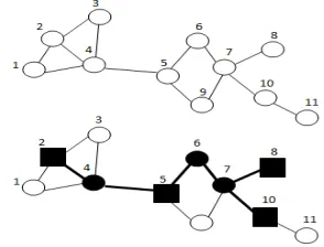
Figure 1: A flat network and its ViBES [20]

Basagni et al. in [6] proposed an algorithm and called it S-DMAC. Backbone nodes are CHs computed by DMAC [5]. Basagni et al. proposed Virtual Backbone for Energy Saving (ViBES) energy efficient construction in [20]. ViBES construction included two important phases: (1) selection of primary ViBES nodes (2) and their interconnection to form a connected backbone. The selection of the ViBES nodes is performed at each node according to the proposed Algorithm in [20]. Figure 1 illustrates the process of selection of ViBES nodes.

404 Energy-Aware Virtual Backbone Tree (EVBT). It chooses only nodes with enough energy levels as the member of the virtual backbone. It also introduced a concept of threshold energy level for members of virtual backbone. Only nodes with energy levels above a predefined threshold can be included in the EVBT. At first, the leader node will check its degree. If degree is greater than one, it verifies whether it can be removed from the graph. When the algorithm terminated that result of iteration is an empty set. At the first iteration, this list is empty. The EVBT is computed at the end of all iterations.

A multiple routing protocol with increasing reliability has been proposed in [21]. This protocol states reliability as probability of success transfer between two nodes in time period t0 to t1:

(1) K is a set of disjoin node routings between source and destination nodes. Also, P(k,t) is defined as reliability of the kth route. Reliability amount of each route is calculated for activity of existing links in the kth route. P(t) states probability of activity at least one route between source and destination nodes [21].

AOMDV protocol in [22] was proposed to identify disjoin links and node routings. All routing tables in this protocol were used to support multiple routing. This protocol saves the distance to source node and the last hop for each route. It prevents iteration cycle in network.

Authors presented a multiple routing protocol for increasing fault tolerance in WSN. This protocol tries to identify partial disjoin routing. For example, the route which differs from the major route in node is a support route. This algorithm was designed based on directed diffusion [23]. The major goal of proposed protocol in [24] is to increase reliability and fault tolerance. This protocol acts to identify disjoin node routes between source and destination nodes. Routing process works with creation of tree via source node in two phases. In the first phase, tree was created with source node as root. Each node identifies a route to destination node via this tree in network. The number of disjoin routes in this phase is equal to the number of tree major branches. In the second phase, each node identifies more disjoin routes via its own neighbors. This extra route is used to increase reliability and fault tolerance.

ReInForm protocol was proposed to guarantee packet sending reliably [25]. This protocol sends

several copies of packet to some of the neighbor nodes. The number of required routes is calculated based on channel error and topologically information of network (the number of hop from source to destination). Energy parameter is not considered in this protocol.

A multiple routing was proposed to decrease energy consumption in WSN. The major goal of designing this protocol is to increase network lifetime via dispatching traffic on more network nodes. In this protocol, network traffic is divided on existing nodes in different routes between each source and destination nodes based on residual energy and received signal power. Also, when the number of active routes between each pair of source and destination nodes was less or equal to two routes, identity phase was started. Otherwise, with failure of a route, network traffic was dispatched again [26].

MCMP protocol considered reliability and link delay between adjacent nodes as routing parameters. Data was sent as multiple routes for increasing reliability. Packets were sent to the nodes which have congestion in this protocol. In that case, the number of sensitive packet decreases [27].

2.2. Learning Automata (LA)

A LA is an adaptive decision making unit that improves its performance by learning how to choose the optimal action from a finite set of allowed actions through repeated interactions with a random environment. The action is chosen at random based on a probability distribution kept over the action-set and at each instant the given action is served as the input to the random environment. The environment responds to the taken action in turn with a reinforcement signal. The action probability vector is updated based on the reinforcement feedback from the environment. The objective of a LA is to find the optimal action from the action-set so that the average penalty received from the environment is minimized [1]-[28-29].

405 environment, and if they vary with time, the environment is called a non stationary environment. The environments depending on the nature of the reinforcement signal β can be classified into P-model, Q-model and S-model. The environments in which the reinforcement signal can only take two binary values 0 and 1 are referred to as P-model environments. Another class of the environment allows a finite number of the values in the interval [0,1] to be taken by the reinforcement signal. Such an environment is referred to as Q-model environment. In S-model environments, the reinforcement signal lies in the interval [a,b]. The relationship between the LA and its random environment has been shown in Figure 2.

Figure 2: The relationship between the learning Automaton and its random environment [1]

LA can be classified into two main families: fixed structure LA and variable structure LA. Variable structure LA is represented by a triple <α, β, T>, where β is the set of inputs, α is the set of actions, and T is learning algorithm. The learning algorithm is a recurrence relation which is used to modify the action probability vector. Let α(k) and p(k) denote the action chosen at instant k and the action probability vector on which the chosen action is based, respectively. The recurrence equation shown by (2) and (3) is a linear learning algorithm by which the action probability vector p is updated. Let α i(k) be the action chosen by the

automaton at instant k. The action probabilities are updated as given in Eq. (2), when the chosen action is rewarded by the environment (i.e., β(n)=0). When the taken action is penalized by the environment, the action probabilities are updated as defined in Eq. (3) (i.e., β(n)= 1) [1]-[28]-[29].

(2)

(3)

Where r is the number of actions that can be chosen by the automaton, a(k) and b(k) denote the reward and penalty parameters and determine the

amount of the increases and decreases of the action probabilities, respectively. If a(k)=b(k), the recurrence Eq. (1) and Eq. (2) are called linear reward-penalty (L R-P) algorithm, if a(k)>> b(k) the

given equations are called linear reward-ɛ penalty

(L R-εP), and finally if b(k)=0 they are called linear

reward-Inaction (L R-I). In the latter case, the action

probability vectors remain unchanged when the taken action is penalized by the environment. In the rest of this section, some convergence results of the LA are summarized.

Definition 1. The average penalty probability M(n), received by a given automaton is defined as M(n)=E[β(n)׀ζ n]=∫ αϵα ζ n (α)f(α), Where ζ:α→[0,1]

specifies the probability of choosing each action αϵα , and ζ n (α) is called the action probability. If

no priori information is available about f, there is no basis for selection of action. So, all the actions are selected with the same probabilities. This automaton is called pure chance automaton and its average penalty is equal to M 0=E[f(α)].

Definition 2. A LA operating in a P-model, Q-model, or S-model environment is said to be expedient if lim n→∞ E[M(n)]< M0.

Expediency means that when automaton updates its action probability function, its average penalty probability decreases. Expediency can also be defined as a closeness of E[M(n)] to f1 = min αf( ).

It is desirable to take an action by which the average penalty can be minimized. In such case, the LA is called optimal.

Definition 3. A LA operating in a P-model, Q-model, or S-model environment is said to be absolutely expedient if E[M(n+1)|p(n)]<M(n) for all n and all pi(n).

Absolute expediency implies that M(n) is a super martingale and E[M(n)] is strictly decreasing for all n in all stationary environments. If M(n)≤M0,

absolute expediency implies expediency.

Definition 4. A LA operating in a P-model, Q-model, or S-model environment is said to be optimal if lim n→∞ E[M(n)]= f1.

406 Definition 5. A LA operating in a P-model, Q-model, or S-model environment is said to be ε-optimal if lim n→∞ E[M(n)] | < f1 +ε, can be obtained

for any ε > 0 by a proper choice of the parameters of the LA. E-optimality implies that the performance of the LA can be made as close to the optimal as desired.

3. THE PROPOSED REERA

We proposed a method to consider a reliable and energy efficient routing in WSNs. Proposed method uses two important factors including residual energy of nodes and reliability function of nodes to select next node in routing formation. This method selects nodes with maximum residual energy and maximum reliability to increase network lifetime. The proposed method is flat and reactive routing, because next node selects using neighborhood information and there is no fixed and predefined structure. This method is a distributed so that each node equip to LA. We assume all nodes are fixed. This algorithm includes of three phases:

3.1. Identity Phase

In this phase, each node identifies its neighbors. Each node sends identity number (ID) and its energy to one-hop neighbors. With the passage of time, energy of nodes decreases. So, we must repeat this phase (e.g. 10 seconds). Here, each node informs of ID and energy and number of its neighbors. Then, each node computes the average of its neighbor energy and is called Eavg. If energy

of nodes are less than Eavg, it will not add to the list

of neighbor nodes. In the next phase, we reward and penalize via Eavg. This phase is repeated only

once in per selection step.

3.2. Learning Phase

In this paper, according to dynamic changes of network and nodes energy situation, LA has been used with variable structure. A network of the LA isomorphic to the UDG was used. It is formed through equipping each node to a LA. At each stage of this approach, the LA randomly chooses one of its actions so that a solution can be found in the routing problem. At first, action probability is equal Pi = 1/n. N is neighbors number of each node I is

action number. At first, a node is selected randomly. Then, the neighbors of this node are selected as next node. At each stage of this approach, we update nodes set in route. The next node is selected based on action probability. This phase continues until a route between source and destination nodes is found. To select nodes in route, we use rewarding and penalizing functions in blow:

If we have Ei ≥ Eavg, selected action must be

rewarded to value of a.

If we have Ei < Eavg, selected action must be

penalized to value of b.

At last, when sum of nodes in and out route was equal to all nodes, current step will be finished. For sending reliable data, the proposed method uses multiple paths and links with high reliability. We show reliability as probability of success transition between two nodes which k is sets of routes between source and destination nodes. The used model is based on [21]. In formula 1, P(k,t) is reliability of the kth route. Reliability of each route be calculated with multiple of active links in each route.

3.3. Monitoring Phase

In this phase, achieved route continues its operation. We use the definition of lifetime in [13]. According to it, lifetime of network is the time that the route is disconnected. Finally, the best route is a route with maximum of residual energy and confidence that is defined as Rreq .

4. SIMULATION EXPERIMENT

To study the performance of the proposed algorithm, we have conducted several simulation experiments (Experiments 1–5) in two groups. The first group of experiments evaluates the results of the proposed algorithm based on reliability, and the second group of experiments is concerned with investigating the impact of the learning rate of algorithm on the CDS size and residual energy.

407 In simulation experiments, wireless sensors communicate through a common broadcast channel using omnidirectional antennas and all sensors have the same radio transmission range R = 20. We consider a WSN with a sink node that is fixed. Sensor nodes are distributed randomly. All sensor nodes are fixed. Also, we use a UDG. For simplicity, we assume that all links are bidirectional and symmetric. In our simulations, the max of iteration is set to 20, and learning rate changes from 0.02 to 0.2. The sensors are randomly distributed in a two-dimensional area of size 100×100 and, and the CDS is formed only on the connected graphs. To simulate, we changed the simulator in [30]. We used energy model that has been presented in [7]. The results shown in Figs. 3–8 are averaged over 100 connected graphs. The simulation square area size, network size, and radio transmission range of sensors are three correlated parameters that affect the network CDS size. In this section, we study how these three parameters affect the backbone (CDS) size, reliability, and residual energy constructed by different algorithms. The Value of parameters can be seen in Table 1.

EXPERIMENT I. To study the impact of the remaining energy on the channel error, we did experiment I. We considered LA on nodes to decreased consumption energy in packets transmission. The number of sending packets for reliability increased with increasing the rate of channel error. For this reason, consumption energy of nodes will increase. Whereas the proposed method considers the residual energy of neighbor nodes to select the next neighbor node, it created a kind of load balance on nodes. So, the value of existing energy in nodes will increase.

EXPERIMENT II. In this experiment, we showed reliability based on rate of channel error in [13] and our method. Due to the fact that the number of deleted packet were increased, the reliability decreases with increasing of channel error. According to the following figure, the reliability of the proposed method is greater than that of another method.

In the second group of simulation studies, we compare the results of the proposed algorithm with those of Acharya et al.’s algorithm [13], Basagni et al.’s algorithm [20], in terms of the network CDS size and residual energy. At each iteration of the simulation scenario which is used in our experiments, the initial dominator nodes are randomly chosen. Then the proposed algorithm chooses the second dominator node according to its action probability vector. Each node forms its

action-set on occasion. This process continues until the network CDS is formed. In all simulations, the constructed CDS is rewarded or penalized with a learning rate of 0.2, 0.02, respectively. The CDS formation process terminates (or simulation stops) when the probability of choosing the CDS exceeds 0.90.

Figure 3 : The Percent Of Residual Energy In Node Based On Error Rate

Figure 4 : Reliability Based On Error

408 connected graphs. Also, the experiment is repeated with LARI where the penalty and reward parameters

are equal the results are depicted in Fig. 6. It can be seen that the CDS size rarely increases and only in some points has peak.

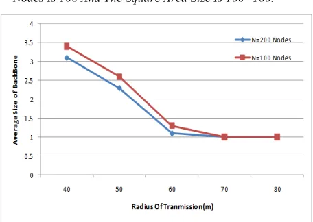
EXPERIMENT IV. To study the effect of the radio transmission range of node on the CDS size, in this experiment, we increased it from 40 to 80 and repeated the same studies as those in experiment I. The number of 100 sensors are randomly distributed in a two-dimensional area of size 100×100 and, and the CDS is formed only on the connected graphs. The results are shown in Fig. 7 and show that the CDS size decreases as the radio transmission range increases. It slightly increases as the network size increases. The results reveal that our proposed algorithm always significantly outperforms the other algorithms in term of the CDS size. We conclude that the variances in the results increases as the learning rate increases. Also, the CDS size is approximately equal when the radio transmission range is 80.

Figure 5: Comparison Of The Average Size For The CDS With The Number Of Nodes, When The Radio Transmission Range Is 40 And The Square Area Size Is

100×100.

EXPERIMENT V. In this experiment, to study the effect of the radio transmission range of the proposed method on the network CDS size, the learning rate is initialized to 0.02 and the CDS size is measured as the network size (number of nodes in network) ranges are 100 and 200 with increment step of 20. The results are depicted in Fig. 8. In these simulation studies, it is assumed that a given number of nodes are randomly and uniformly distributed in a square simulation area of size 100×100 units. As shown in Fig. 8, the network CDS size decreases as the radio transmission range of algorithm increases. Also, the network CDS size

with 200 nodes is better than with 100 nodes. It is clear that the more nodes, the better choice.

Figure 6 : Comparison Of The Average Size For The CDS, When The Radio Transmission Range Is 40 And LA Is With LARIAnd The Square Area Size Is 100×100.

Figure 7: Comparison Of The Average Size For The CDS With The Radius Of Transmission, When The Number Of

Nodes Is 100 And The Square Area Size Is 100×100.

Figure 8: The Average CDS Size In Proposed Algorithm When The Number Of Nodes Is 100 And 200 And The

409 Table 1: The Values Of Used Parameters In Simulator.

Value

Parameter Type

100, 200 The number of

nodes

100m

×

1j Initial energy of

each node

50nj/bit

E

100pj/bit/m2

E

20 bit The size of packet

20m Transmission range

5. CONCLUSION

The routing algorithm has proven to be an effective construction to solve a variety of problems in WSNs. we proposed a new routing algorithm to improve reliability and lifetime in WSNs. In this paper, we proposed a reliable and energy efficient routing algorithm in which by finding a solution to the CDS problem. Reducing the rebroadcasts due to sending the messages along the CDS alleviates the notorious broadcast storm problem in sensor networks. The proposed algorithm could be also used in energy efficient routing algorithm, where the only group members need to be dominated by the CDS. We compared the results of our proposed algorithm with the best-known routing algorithm and showed that our algorithm always outperforms in terms of the remaining energy, size of CDS, and reliability. Our algorithm increases reliability, decreases the overall energy consumption and increases network effective lifetime. The experimental results showed that our proposed algorithm significantly outperforms Wu and Li algorithm in terms of the remaining energy, size of CDS, and reliability.

REFRENCES:

[1] J. Akbari Torkestani, M.R. Meybodi, “An intelligent backbone formation algorithm for wireless ad networks based on distributed learning automata”, Computer Network Journal vol. 54, 2010, pp. 826–843.

[2] S. Hussain, M.I. Shafique, and L.T. Yang, “Constructing a CDS-Based Network Backbone for Energy Efficiency in Industrial Wireless Sensor Network”, Proceeding of HPCC, 2010, pp.322-328.

[3] S. Basagni, R. Petroccia, C.H. Petrioli, “Efficiently reconfigurable backbones for wireless sensor networks”, Computer and Communication Journal, vol. 31, no. 4, 2008, pp. 668-698.

[4] M. Rai, S.H. Verma, and S.H. Tapaswi, “A Power Aware Minimum Connected Dominating Set for Wireless Sensor Networks”, Journal of network, vol. 4, no. 6, 2009.

[5] S. Basagni, “Distributed clustering for ad hoc networks”, Proceeding IEEE, The Fourth International Symposium Parallel Arch Algorithm Network, (I-SPAN '99), 1999, pp.310 -315.

[6] S. Basagni, A. Carosi, and C.H. Petrioli, ”Sensor-DMAC: Dynamic Topology Control for Wireless Sensor Networks”, Proceeding IEEE VTC Fall, 2004, pp. 2930-2935.

[7] W.R. Heinzelman, A. Chandrakasan, and H. Balakrishnand, “Energy-Efficient communication Protocol for Wireless Microsensor Networks”, Proceedings of the 33rd Hawaii International Conference on System and Sciences (HICSS), vol. 8, 2000, pp. 8020-8032.

[8] B. Jeremy, D. Min, and T. Andrew and C. Xiuzhen, “Connected Dominating Set in Sensor Networks and MANETs”, Handbook of Combinatorial Optimization, Springer Journal, 2004.

[9] R. Asgarnezhad, J. Akbari Torkestani, “A Survey on Backbone Formation Algorithms for Wireless Sensor Networks”, Austrasian Telecommunication Network and Application conference, (ATNAC), IEEE, pp.1-4.

[10] R. Asgarnezhad, J. Akbari Torkestani, “Connected Dominating Set Problem and its Application to ireless Sensor Networks”, The First International Conference Advanced Communication and Computer (INFOCOMP) 2011, pp.46–51.

[11] Z. Liu, B. Wang, and Q. Tang, “Approximation Two Independent Sets Based Connected Dominating Set Construction Algorithm for Wireless Sensor Networks”, Journal of Information Technology, vol. 9, no. 5, 2010, pp. 864-876.

[12] M.T. Thai, W. Feng, and L. Dan and Z. Shiwei and D. Ding-Zhu, “Connected dominating sets in wireless networks with different transmission ranges”, IEEE Transaction on Mobile Computer, vol. 6, 2007, 721-730.

410 [14] S. Butenko, X. Cheng, and A. Carlos and C.

Oliveira C and P.M. Pardalos, “A New Heuristic For The Minimum Connected Dominating Set Problem On Ad Hoc Wireless Networks”, Recent Developments in Cooperative Control and Optimization, Kluwer Academic Publishers, 2004, pp.61-73.

[15] X. Cheng, M. Ding, and D. Chen, “An approximation algorithm for connected dominating set in ad hoc networks”, Proceeding of International Workshop on Theoretical Aspects of Wireless Ad Hoc, Sensor, and Peer-to-Peer Network, (TAWN), 2004.

[16] B. Das, V. Bharghavan, “Routing in Ad-Hoc Networks Using Minimum Connected Dominating Sets”, International Conference on Communication, (ICC), vol. 1, 1997, pp. 376-380.

[17] S. Guha, S. Khuller, ‘Approximation algorithms for connected dominating sets”, Algorithmic Journal, vil. 20, no. 4, 1998, pp. 374-387. [18] J. Wu, H. Li, “On calculating connected

dominating set for efficient routing in ad hoc wireless networks”, Proceeding of ACMDIALM, 1999, pp.7–14.

[19] R. Xie, D. Qi, and Y. Li and J.Z. Wang, “A novel distributed MCDS approximation algorithm for wireless sensor networks”, Mobile & Wireless Communication Journal, vol. 9, no. 3, 2009, pp. 427–437.

[20] S. Basagni, M. Elia, R.Ghosh, “ViBES: virtual backbone for energy saving in wireless sensor networks”, Military Communication Conference (MILCOM), IEEE Press, vol. 3, 2004, pp. 1240 – 1246.

[21] R. Leung, J. Liu, and E. Poon and A.L.C. Chan, B. Li, “MP-DSR: a QoS-aware Multi-Path Dynamic Source Routing Protocol for Wireless ad-hoc Networks”, Local Computer Network Journal IEEE, 2001, pp.132-141.

[22] M. Marina, S. Das, “On-demand multipath Distance Vector Routing in Ad Hoc Networks”, Ninth International Conference on Network Protocols, (ICNP), 2001.

[23] D. Ganesan, R. Govindan, and S. Shenke and D. Estrin, “Highly-Resilient Energy-Efficient Multipath Routing in wireless Sensor Networks”, ACM SIGMOBILE Mobile Computer and Communication Review, vol. 5, no. 4, 2001, pp. 11-25.

[24] W. Lou, “An Efficient N-to-1 Multipath Routing Protocol in Wireless Sensor Networks”, IEEE International Conference on Mobile Ad hoc and Sensor System, vol. 7, no. 7, 2005.

[25] B. Deb, S. Bhatnagar, and B. Nath, “ReInForM: Reliableinformation forwarding using multiple paths in sensor networks”,in 28th Annual IEEE International Conference on Local Computer Networks, 2003, pp.406-415.

[26] R. Vidhyapriya, P.T. Vanathi, “Energy Efficient Adaptive Multipath Routing for Wireless Sensor Networks”, IAENG International Journal of Computer Science, 2007.

[27] X. Huang, Y. Fang, “Multiconstrained QoS multipath routingin wireless sensor networks”, Wireless Network Journal, vol. 14, no. 4, 2007, pp. 465-478.

[28] H. Beigy, M.R. Meybodi, “Utilizing distributed learning automata to solve stochastic shortest path problems”, International Journal Uncertainty, Fuzziness and Knowledge-Based Systems, vol. 14, 2006, pp. 591-615.

[29] K.S. Narendra, K.S. Thathacher, “Learning Automata: An Introduction”, New York, Prentice-Hall, 1989.