International Journal of Industrial Engineering Computations 7 (2016) 295–308
Contents lists available at GrowingScience
International Journal of Industrial Engineering Computations
homepage: www.GrowingScience.com/ijiec
A hybrid algorithm for stochastic single-source capacitated facility location problem with service level requirements
Hosseinali Salemia*
School of industrial and information engineering, Politecnico di Milano, Piazza Leonardo da Vinci, 32, 20133, Milano, Italy
C H R O N I C L E A B S T R A C T
Article history: Received July 21 2015 Received in Revised Format August 16 2015
Accepted October 8 2015 Available online October 8 2015
Facility location models are observed in many diverse areas such as communication networks, transportation, and distribution systems planning. They play significant role in supply chain and operations management and are one of the main well-known topics in strategic agenda of contemporary manufacturing and service companies accompanied by long-lasting effects. We define a new approach for solving stochastic single source capacitated facility location problem (SSSCFLP). Customers with stochastic demand are assigned to set of capacitated facilities that are selected to serve them. It is demonstrated that problem can be transformed to deterministic Single Source Capacitated Facility Location Problem (SSCFLP) for Poisson demand distribution. A hybrid algorithm which combines Lagrangian heuristic with adjusted mixture of Ant colony and Genetic optimization is proposed to find lower and upper bounds for this problem. Computational results of various instances with distinct properties indicate that proposed solving approach is efficient.
© 2016 Growing Science Ltd. All rights reserved
Keywords:
Supply chain management Lagrangian
heuristic
Ant colony optimization Genetic optimization Service level
Stochastic facility location problem Poisson distribution Hybrid Algorithm
1. Introduction
A segment of supply chain management is dedicated to facility location problems (FLP). Given a set of potential locations of facilities (e.g. plants, warehouses) and a set of demand points, facility location problem is to find locations of facilities in a way that total cost of opening and allocation of customers for satisfying their demand is minimized. These problems may be seen as the most critical and significant decisions in building an efficient supply chain since they are fixed and difficult to change even in the intermediate term. The location of a multibillion-dollar facility cannot be changed as a result of changes in customer demands, raw material price or transportation rates. There are different categories of facility location problem relying on restrictions assumption. One concern in FLP is the capacity of each facility for serving its assigned demand points. While in the uncapacitated facility location problem, capacity of each facility is assumed to be infinite, in capacitated facility location problem (CFLP), each facility has a finite capacity. Single Source Capacitated Facility Location Problem (SSCFLP) which is proven to * Corresponding author. Tel: +39-3207761926
belong to category of NP-hard problems, is a subset of CFLP where each customer receives all its demand from just one opened facility. SSCFLP is the opposite point of multi-sourcing capacitated problems. In real world, demand of customers are not pre-determined and definite, but stochastic and indecisive. Hence, facilities should have sufficient capacity to cope with uncertainties with a degree of reliability level.
Following model is Stochastic Single Source Capacitated Facility Location Problem (SSSFLP) that determines which facilities should be opened and which demand points are allocated to each of them in a way that total cost is minimized:
Notation
𝐼𝐼 {1,2, … ,𝑚𝑚} 𝑠𝑠𝑠𝑠𝑠𝑠𝑜𝑜𝑜𝑜𝑐𝑐𝑐𝑐𝑐𝑐𝑐𝑐𝑐𝑐𝑐𝑐𝑐𝑐𝑠𝑠𝑠𝑠𝑜𝑜𝑐𝑐𝑐𝑐𝑐𝑐𝑓𝑓𝑐𝑐𝑠𝑠𝑐𝑐𝑠𝑠𝑠𝑠 𝐽𝐽 {1,2, … ,𝑐𝑐} 𝑠𝑠𝑠𝑠𝑠𝑠𝑜𝑜𝑜𝑜𝑐𝑐𝑠𝑠𝑚𝑚𝑐𝑐𝑐𝑐𝑐𝑐𝑝𝑝𝑜𝑜𝑐𝑐𝑐𝑐𝑠𝑠𝑠𝑠
Decision variables
𝑦𝑦𝑖𝑖 𝑐𝑐𝑠𝑠𝑠𝑠𝑠𝑠𝑑𝑑𝑚𝑚𝑐𝑐𝑐𝑐𝑠𝑠𝑠𝑠𝑤𝑤ℎ𝑠𝑠𝑠𝑠ℎ𝑠𝑠𝑑𝑑𝑜𝑜𝑐𝑐𝑐𝑐𝑐𝑐𝑓𝑓𝑐𝑐𝑠𝑠𝑦𝑦𝑐𝑐𝑐𝑐𝑠𝑠𝑜𝑜𝑝𝑝𝑠𝑠𝑐𝑐𝑠𝑠𝑐𝑐𝑜𝑜𝑑𝑑𝑐𝑐𝑜𝑜𝑠𝑠
𝑋𝑋𝑖𝑖𝑖𝑖 𝑐𝑐𝑠𝑠𝑠𝑠𝑠𝑠𝑑𝑑𝑚𝑚𝑐𝑐𝑐𝑐𝑠𝑠𝑠𝑠𝑤𝑤ℎ𝑠𝑠𝑠𝑠ℎ𝑠𝑠𝑑𝑑𝑐𝑐𝑠𝑠𝑚𝑚𝑐𝑐𝑐𝑐𝑐𝑐𝑝𝑝𝑜𝑜𝑐𝑐𝑐𝑐𝑠𝑠𝑗𝑗𝑐𝑐𝑠𝑠𝑐𝑐𝑠𝑠𝑠𝑠𝑐𝑐𝑎𝑎𝑐𝑐𝑠𝑠𝑐𝑐𝑠𝑠𝑜𝑜𝑜𝑜𝑐𝑐𝑐𝑐𝑐𝑐𝑓𝑓𝑐𝑐𝑠𝑠𝑦𝑦𝑐𝑐𝑜𝑜𝑑𝑑𝑐𝑐𝑜𝑜𝑠𝑠
Formulation
(𝕾𝕾) 𝑧𝑧=𝑚𝑚𝑐𝑐𝑐𝑐 � 𝑜𝑜𝑖𝑖𝑦𝑦𝑖𝑖 + � � 𝑐𝑐𝑖𝑖𝑖𝑖𝑋𝑋𝑖𝑖𝑖𝑖 𝑛𝑛
𝑖𝑖=1 𝑚𝑚
𝑖𝑖=1 𝑚𝑚
𝑖𝑖=1 Subject to:
� 𝑋𝑋𝑖𝑖𝑖𝑖 = 1 𝑗𝑗 = 1,2, … , n 𝑚𝑚
𝑖𝑖=1 (1)
𝑝𝑝𝑑𝑑𝑜𝑜𝑝𝑝 (� 𝑐𝑐𝑖𝑖𝑋𝑋𝑖𝑖𝑖𝑖 ≤ 𝑄𝑄𝑖𝑖𝑦𝑦𝑖𝑖) ≥ 𝛼𝛼𝑖𝑖 𝑐𝑐 = 1,2, … ,𝑚𝑚 𝑛𝑛
𝑖𝑖=1 (2)
𝑋𝑋𝑖𝑖𝑖𝑖 ≤ 𝑦𝑦𝑖𝑖 𝑐𝑐= 1,2, … ,𝑚𝑚 𝑗𝑗 = 1,2, … , n (3)
𝑦𝑦𝑖𝑖 = �0,1, 𝑐𝑐𝑜𝑜𝑜𝑜𝑠𝑠ℎ𝑠𝑠𝑑𝑑𝑤𝑤𝑐𝑐𝑠𝑠𝑠𝑠𝑜𝑜𝑐𝑐𝑐𝑐𝑐𝑐𝑓𝑓𝑐𝑐𝑠𝑠𝑦𝑦𝑐𝑐𝑐𝑐𝑠𝑠𝑜𝑜𝑝𝑝𝑠𝑠𝑐𝑐𝑠𝑠𝑐𝑐 𝑐𝑐 = 1,2, … ,𝑚𝑚 (4)
𝑋𝑋𝑖𝑖𝑖𝑖 = �0,1, 𝑐𝑐𝑜𝑜𝑜𝑜𝑠𝑠ℎ𝑠𝑠𝑑𝑑𝑤𝑤𝑐𝑐𝑠𝑠𝑠𝑠𝑜𝑜𝑐𝑐𝑐𝑐𝑐𝑐𝑓𝑓𝑐𝑐𝑠𝑠𝑦𝑦𝑐𝑐𝑐𝑐𝑠𝑠𝑐𝑐𝑠𝑠𝑠𝑠𝑐𝑐𝑎𝑎𝑐𝑐𝑠𝑠𝑐𝑐𝑠𝑠𝑜𝑜𝑐𝑐𝑠𝑠𝑚𝑚𝑐𝑐𝑐𝑐𝑐𝑐𝑝𝑝𝑜𝑜𝑐𝑐𝑐𝑐𝑠𝑠𝑗𝑗 𝑐𝑐= 1,2, … ,𝑚𝑚 𝑗𝑗 = 1,2, … , n (5) The decision is about selecting a set of facilities among 𝑚𝑚 candidates and assignment of each demand point 𝑗𝑗 (𝑗𝑗 = 1,2, … ,𝑐𝑐) to exactly one opened facility 𝑐𝑐. The objective function minimizes opened facilities fixed costs 𝑜𝑜𝑖𝑖 and serving costs 𝑐𝑐𝑖𝑖𝑖𝑖 related to assignment of each customer 𝑗𝑗 to a unique facility
assigned to that facility requested. Constraint (3) certifies that assignment of demand points to a facility takes place just if that facility is opened. Constraints (4) and (5) show that 𝑦𝑦𝑖𝑖 and 𝑋𝑋𝑖𝑖𝑖𝑖 are binary variables that can be zero or one.
The paper is organized in 6 sections. Section 2 reviews the literature about different methods of solving facility location problems. Section 3 examines the case of Poisson demand distribution. Section 4 introduces the novel and state-of-the-art hybrid algorithm to solve SSSCFLP. In section 5 computational results are provided. Conclusion is presented in section 6.
2. Literature review
Different approaches for solving SSCFLP is extant in literature. Neebe and Rao (1983) formulate SSCLP as a set partitioning problem and solve it by a column-generating branch and bound procedure. Bounds are obtained by using linear relaxation. Due to the high probability of having integer solutions with the linear program, they observe that the tree search is not very large.
The most successful approach known to be is Lagrangian heuristic. The basis of these heuristics is a combination of Lagrangian relaxation and methods for solving the Lagrangian dual problem with the aim of finding lower and upper bounds of optimal solution. Beasley (1993) introduces a framework to develop Lagrangian heuristics based on Lagrangian relaxation and subgradient optimization for location problems in which both capacity and demand points constraints are relaxed and dualized. His work provides efficient solution for different types of location problems like uncapacitated, p-median, capacitated and single source capacitated facility location problems. Holmberg et al. (1999) propose Lagrangian heuristic involving Lagrangian relaxation, subgradient optimization and primal heuristic within a branch-and-bound framework to solve SSCFLP with high quality and robustness. The primal heuristic is based on solving a sequence of related matching problems and is incorporated into Lagrangian heuristic. Tragantalerngsak et al. (2000) present a Lagrangian relaxation-based branch-and-bound algorithm for solving a particular type of FLP in which two echelons of facilities exist. Only one facility in the first echelon can serve each facility of the second echelon which has a limited capacity and each demand point receives its orders from just one facility in the second echelon. Klincewicz and Luss. (1986) use Lagrangian heuristic to solve SSCFLP by relaxing capacity constraints, obtaining uncapacitated facility location as a subproblem and using dual ascent algorithm. A heuristic based on cost differentials is applied to decrease cost of solution obtained in Lagrangian phase. Barcelo and Casanovas (1984) present a Lagrangian heuristic solution in which customer assignment constraints are relaxed and series of knapsack problems are generated. The proposed Lagrangian heuristic involves two sections of facility location selection and demand points allocation. In assignment of customers to opened facilities, regret heuristic is used.
The objective of this work is to develop a method and algorithm to provide good solutions for Stochastic Single Source Capacitated Facility Location Problem (SSSCFLP). Poisson distribution demand is considered and its equivalent deterministic model and proposed solution algorithm is described.
3. Poisson demand
We consider Poisson demand distribution where demand node j has mean 𝜆𝜆𝑖𝑖 (𝑗𝑗 ∈ 𝐽𝐽). This distribution function for customer demand can be observed in medical, emergency or telecommunication services. Now, we try to change the stochastic problem (𝕾𝕾) to deterministic one as done in C.K.Y. (Lin, 2009). Since sum of a set of Poisson random variables is a Poisson variable, ∑𝑛𝑛𝑖𝑖=1𝑐𝑐𝑖𝑖𝑋𝑋𝑖𝑖𝑖𝑖, which is the total demand assigned to facility 𝑐𝑐can be modeled by a Poisson variable of mean ∑𝑛𝑛𝑖𝑖=1𝜆𝜆𝑖𝑖𝑋𝑋𝑖𝑖𝑖𝑖. So, Eq. (2) in (𝕾𝕾) , can be rewritten as:
� 𝑠𝑠−(∑𝑗𝑗=1𝑛𝑛 𝜆𝜆𝑗𝑗𝑋𝑋𝑖𝑖𝑗𝑗) (∑ 𝜆𝜆𝑖𝑖𝑋𝑋𝑖𝑖𝑖𝑖 )
𝑛𝑛
𝑖𝑖=1 𝑘𝑘
𝑘𝑘! 𝑄𝑄𝑖𝑖𝑦𝑦𝑖𝑖
𝑘𝑘=0
≥ 𝛼𝛼𝑖𝑖 𝑐𝑐= 1,2, … ,𝑚𝑚 (6)
Assume we have a Poisson variable 𝑥𝑥 whose mean is the largest value satisfying condition
𝑝𝑝𝑑𝑑𝑜𝑜𝑝𝑝 (𝑥𝑥 ≤ 𝑄𝑄𝑖𝑖) ≥ 𝛼𝛼𝑖𝑖. We denote mean of 𝑥𝑥 by 𝑝𝑝𝑖𝑖 and vary it until 𝑝𝑝𝑑𝑑𝑜𝑜𝑝𝑝 (𝑥𝑥 ≤ 𝑄𝑄𝑖𝑖)≅ 𝛼𝛼𝑖𝑖 is obtained.
𝑝𝑝𝑖𝑖, which is a function of 𝑄𝑄𝑖𝑖 and 𝛼𝛼𝑖𝑖, can be easily found by try and error method. In this way we can
rewrite Eq. (6) as:
� 𝜆𝜆𝑖𝑖𝑋𝑋𝑖𝑖𝑖𝑖 𝑛𝑛
𝑖𝑖=1
≤ 𝑝𝑝𝑖𝑖𝑦𝑦𝑖𝑖 𝑐𝑐= 1,2, … ,𝑚𝑚
(7) If we replace Eq. (7) with Eq. (2), stochastic model is changed to a deterministic one:
(𝕯𝕯) 𝑧𝑧= 𝑚𝑚𝑐𝑐𝑐𝑐 � 𝑜𝑜𝑖𝑖𝑦𝑦𝑖𝑖 + � � 𝑐𝑐𝑖𝑖𝑖𝑖𝑋𝑋𝑖𝑖𝑖𝑖 𝑛𝑛
𝑖𝑖=1 𝑚𝑚
𝑖𝑖=1 𝑚𝑚
𝑖𝑖=1
subject to
� 𝑋𝑋𝑖𝑖𝑖𝑖 = 1 j = 1,2, … , n 𝑚𝑚
𝑖𝑖=1
� 𝜆𝜆𝑖𝑖𝑋𝑋𝑖𝑖𝑖𝑖 𝑛𝑛
𝑖𝑖=1
≤ 𝑝𝑝𝑖𝑖𝑦𝑦𝑖𝑖 𝑐𝑐 = 1,2, … ,𝑚𝑚
𝑋𝑋𝑖𝑖𝑖𝑖 ≤ 𝑦𝑦𝑖𝑖 𝑐𝑐= 1,2, … ,𝑚𝑚 j = 1,2, … , n
𝑦𝑦𝑖𝑖 = �0,1, 𝑐𝑐𝑜𝑜𝑜𝑜𝑠𝑠ℎ𝑠𝑠𝑑𝑑𝑤𝑤𝑐𝑐𝑠𝑠𝑠𝑠𝑜𝑜𝑐𝑐𝑐𝑐𝑐𝑐𝑓𝑓𝑐𝑐𝑠𝑠𝑦𝑦𝑐𝑐𝑐𝑐𝑠𝑠𝑜𝑜𝑝𝑝𝑠𝑠𝑐𝑐𝑠𝑠𝑐𝑐 𝑐𝑐 = 1,2, … ,𝑚𝑚
𝑋𝑋𝑖𝑖𝑖𝑖 = �0,1, 𝑐𝑐𝑜𝑜𝑜𝑜𝑠𝑠ℎ𝑠𝑠𝑑𝑑𝑤𝑤𝑐𝑐𝑠𝑠𝑠𝑠𝑜𝑜𝑐𝑐𝑐𝑐𝑐𝑐𝑓𝑓𝑐𝑐𝑠𝑠𝑦𝑦𝑐𝑐𝑐𝑐𝑠𝑠𝑐𝑐𝑠𝑠𝑠𝑠𝑐𝑐𝑎𝑎𝑐𝑐𝑠𝑠𝑐𝑐𝑠𝑠𝑜𝑜𝑐𝑐𝑠𝑠𝑚𝑚𝑐𝑐𝑐𝑐𝑐𝑐𝑝𝑝𝑜𝑜𝑐𝑐𝑐𝑐𝑠𝑠𝑗𝑗 𝑐𝑐= 1,2, … ,𝑚𝑚 j = 1,2, … , n
If we solve (𝕯𝕯), it will guarantee that constraint ∑𝑖𝑖=1𝑛𝑛 𝜆𝜆𝑖𝑖𝑋𝑋𝑖𝑖𝑖𝑖 ≤ 𝑝𝑝𝑖𝑖𝑦𝑦𝑖𝑖 is satisfied and since 𝑝𝑝𝑖𝑖 is the
largest value satisfying 𝑝𝑝𝑑𝑑𝑜𝑜𝑝𝑝 (𝑥𝑥 ≤ 𝑄𝑄𝑖𝑖) ≅ 𝛼𝛼𝑖𝑖 , it assures that with probability higher than 𝛼𝛼𝑖𝑖 ,
4. Hybrid algorithm (Combination of Lagrangian Heuristic and adjusted mixture of Ant colony and Genetic Metaheuristics optimization algorithm)
Proposed algorithm combines well-known Lagrangian heuristic with adjusted mixture of Ant colony and Genetic Metahuristics to solve (𝕯𝕯). The main idea behind this algorithm is to obtain a lower bound through Lagrangian relaxation which is enclosed by subgradient optimization method with the aim of generating a sequence of Lagrangian multipliers and acquiring highest possible lower bound. At each iteration of subgradient optimization the adjusted mixture of Ant colony and Genetic Metahuristics are applied to construct a feasible solution and possibly generate better upper bounds. These steps are provided in three phases as follows:
Phase 1. Lagrangian Relaxation: with Lagrangian relaxation, lower bounds on the optimal objective function of (𝕯𝕯) will be produced.
Phase 2. Subgradient optimization: in this phase Lagrangian dual is solved, lower bounds will be improved and Lagrangian multiplier is updated.
Phase 3. Adjusted mixture of Ant colony and Genetic Metaheuristics optimization: In this phase we find feasible solutions as well as possibly update upper bounds on the objective function of (𝕯𝕯).
In the following each phase will be described in detail: Phase1. Lagrangian Relaxation
Lagrangian relaxation is a technique to obtain a relaxed problem, called Lagrangian subproblem, which is easier to be solved than original problem. The basic idea is to remove or relax set of problem constraints and put them into objective function assigned with weights (Lagrangian multiplier). Each weight is the representation of a penalty which is added to solution that does not satisfy the set of relaxed constraints. Since problem (𝕯𝕯) is a minimization problem, the objective value of its relaxed problem provides a lower bound for it.
We relax constraint ∑𝑖𝑖=1𝑚𝑚 𝑋𝑋𝑖𝑖𝑖𝑖 = 1 (𝑗𝑗 = 1,2, … ,𝑐𝑐) of (𝕯𝕯) with associated Lagrangian multiplier 𝜇𝜇𝑖𝑖 (𝜇𝜇𝑖𝑖 ≥ 0) :
(𝕷𝕷) 𝑧𝑧(𝜇𝜇) =𝑚𝑚𝑐𝑐𝑐𝑐 � 𝑜𝑜𝑖𝑖𝑦𝑦𝑖𝑖 𝑚𝑚
𝑖𝑖=1
+ � � 𝑐𝑐𝑖𝑖𝑖𝑖𝑋𝑋𝑖𝑖𝑖𝑖+ � 𝜇𝜇𝑖𝑖(1− � 𝑋𝑋𝑖𝑖𝑖𝑖)
𝑚𝑚
𝑖𝑖=1 𝑛𝑛
𝑖𝑖=1 𝑛𝑛
𝑖𝑖=1 𝑚𝑚
𝑖𝑖=1
subject to
� 𝜆𝜆𝑖𝑖𝑋𝑋𝑖𝑖𝑖𝑖 𝑛𝑛
𝑖𝑖=1
≤ 𝑝𝑝𝑖𝑖𝑦𝑦𝑖𝑖 𝑐𝑐= 1,2, … ,𝑚𝑚
𝑋𝑋𝑖𝑖𝑖𝑖 ≤ 𝑦𝑦𝑖𝑖 𝑐𝑐= 1,2, … ,𝑚𝑚 𝑗𝑗 = 1,2, … ,𝑐𝑐
𝑦𝑦𝑖𝑖 = �1,0, 𝑜𝑜𝑠𝑠ℎ𝑠𝑠𝑑𝑑𝑤𝑤𝑐𝑐𝑠𝑠𝑠𝑠𝑐𝑐𝑜𝑜𝑜𝑜𝑐𝑐𝑐𝑐𝑐𝑐𝑓𝑓𝑐𝑐𝑠𝑠𝑦𝑦𝑐𝑐𝑐𝑐𝑠𝑠𝑜𝑜𝑝𝑝𝑠𝑠𝑐𝑐𝑠𝑠𝑐𝑐 𝑐𝑐 = 1,2, … ,𝑚𝑚
𝑋𝑋𝑖𝑖𝑖𝑖 = �0,1, 𝑐𝑐𝑜𝑜𝑜𝑜𝑠𝑠ℎ𝑠𝑠𝑑𝑑𝑤𝑤𝑐𝑐𝑠𝑠𝑠𝑠𝑜𝑜𝑐𝑐𝑐𝑐𝑐𝑐𝑓𝑓𝑐𝑐𝑠𝑠𝑦𝑦𝑐𝑐𝑐𝑐𝑠𝑠𝑐𝑐𝑠𝑠𝑠𝑠𝑐𝑐𝑎𝑎𝑐𝑐𝑠𝑠𝑐𝑐𝑠𝑠𝑜𝑜𝑐𝑐𝑠𝑠𝑚𝑚𝑐𝑐𝑐𝑐𝑐𝑐𝑝𝑝𝑜𝑜𝑐𝑐𝑐𝑐𝑠𝑠𝑗𝑗 𝑐𝑐= 1,2, … ,𝑚𝑚 𝑗𝑗 = 1,2, … ,𝑐𝑐
(𝓚𝓚) 𝑘𝑘 =𝑚𝑚𝑐𝑐𝑐𝑐 ��𝑐𝑐𝑖𝑖𝑖𝑖 − 𝜇𝜇𝑖𝑖�𝑋𝑋𝑖𝑖𝑖𝑖 𝑛𝑛
𝑖𝑖=1
subject to
� 𝜆𝜆𝑖𝑖𝑋𝑋𝑖𝑖𝑖𝑖 𝑛𝑛
𝑖𝑖=1
≤ 𝑝𝑝𝑖𝑖𝑦𝑦𝑖𝑖 𝑐𝑐= 1,2, … ,𝑚𝑚
𝑋𝑋𝑖𝑖𝑖𝑖 = �0,1, 𝑐𝑐𝑜𝑜𝑜𝑜𝑠𝑠ℎ𝑠𝑠𝑑𝑑𝑤𝑤𝑐𝑐𝑠𝑠𝑠𝑠𝑜𝑜𝑐𝑐𝑐𝑐𝑐𝑐𝑓𝑓𝑐𝑐𝑠𝑠𝑦𝑦𝑐𝑐𝑐𝑐𝑠𝑠𝑐𝑐𝑠𝑠𝑠𝑠𝑐𝑐𝑎𝑎𝑐𝑐𝑠𝑠𝑐𝑐𝑠𝑠𝑜𝑜𝑐𝑐𝑠𝑠𝑚𝑚𝑐𝑐𝑐𝑐𝑐𝑐𝑝𝑝𝑜𝑜𝑐𝑐𝑐𝑐𝑠𝑠𝑗𝑗 𝑐𝑐= 1,2, … ,𝑚𝑚 𝑗𝑗 = 1,2, … ,𝑐𝑐
After solving (𝓚𝓚), the term 𝑜𝑜𝑖𝑖+∑ �𝑐𝑐𝑛𝑛𝑖𝑖=1 𝑖𝑖𝑖𝑖− 𝜇𝜇𝑖𝑖�𝑋𝑋𝑖𝑖𝑖𝑖 which can be noticed as reduced cost for 𝑦𝑦𝑖𝑖 is calculated for each and every facility. If it is lower than zero, then 𝑦𝑦𝑖𝑖 = 1 and 𝑋𝑋𝑖𝑖𝑖𝑖 are the quantities that have been obtained from knapsack problem. Otherwise, both 𝑦𝑦𝑖𝑖 and 𝑋𝑋𝑖𝑖𝑖𝑖 will be zero:
𝑐𝑐𝑜𝑜𝑜𝑜𝑖𝑖 +��𝑐𝑐𝑖𝑖𝑖𝑖 − 𝜇𝜇𝑖𝑖(1)�𝑋𝑋𝑖𝑖𝑖𝑖 𝑛𝑛
𝑖𝑖=1
< 0 𝑦𝑦𝑖𝑖 = 1 ,𝑋𝑋𝑖𝑖𝑖𝑖 =𝑄𝑄𝑄𝑄𝑐𝑐𝑐𝑐𝑠𝑠𝑐𝑐𝑠𝑠𝑐𝑐𝑠𝑠𝑠𝑠𝑜𝑜𝑝𝑝𝑠𝑠𝑐𝑐𝑐𝑐𝑐𝑐𝑠𝑠𝑐𝑐𝑜𝑜𝑑𝑑𝑜𝑜𝑚𝑚 (𝒦𝒦)
𝑐𝑐𝑜𝑜𝑜𝑜𝑖𝑖 +��𝑐𝑐𝑖𝑖𝑖𝑖 − 𝜇𝜇𝑖𝑖(1)�𝑋𝑋𝑖𝑖𝑖𝑖 𝑛𝑛
𝑖𝑖=1
> 0 𝑦𝑦𝑖𝑖 = 0 ,𝑋𝑋𝑖𝑖𝑖𝑖 = 0
Proof
We know that 𝑜𝑜𝑖𝑖≥ 0 and ∑𝑛𝑛𝑖𝑖=1𝑐𝑐𝑖𝑖𝑖𝑖𝑋𝑋𝑖𝑖𝑖𝑖≥0. So, if 𝑜𝑜𝑖𝑖 +∑𝑛𝑛𝑖𝑖=1𝑐𝑐𝑖𝑖𝑖𝑖𝑋𝑋𝑖𝑖𝑖𝑖 − ∑𝑖𝑖=1𝑛𝑛 𝜇𝜇𝑖𝑖𝑋𝑋𝑖𝑖𝑖𝑖 < 0 then ∑𝑛𝑛𝑖𝑖=1𝜇𝜇𝑖𝑖𝑋𝑋𝑖𝑖𝑖𝑖 > 0. We also know that Lagrangian multiplier 𝜇𝜇𝑖𝑖 ≥0. Therefore 𝑋𝑋𝑖𝑖𝑖𝑖 > 0. 𝑋𝑋𝑖𝑖𝑖𝑖 is a binary variable which can be zero or one and if it is more than zero it has to be one. Being 𝑋𝑋𝑖𝑖𝑖𝑖 = 1 indicates that facility 𝑐𝑐 is opened so 𝑦𝑦𝑖𝑖 = 1.
If 𝑜𝑜𝑖𝑖 +∑𝑛𝑛𝑖𝑖=1𝑐𝑐𝑖𝑖𝑖𝑖𝑋𝑋𝑖𝑖𝑖𝑖 − ∑𝑖𝑖=1𝑛𝑛 𝜇𝜇𝑖𝑖𝑋𝑋𝑖𝑖𝑖𝑖 > 0, it is not beneficial to open facility 𝑐𝑐 so 𝑦𝑦𝑖𝑖 = 0 and consequently
𝑋𝑋𝑖𝑖𝑖𝑖 = 0. Lower bound
The optimal value of objective function (𝕷𝕷) which is the lower bound will be:
𝑧𝑧(𝜇𝜇) =� ( 𝑜𝑜𝑖𝑖𝑦𝑦�𝚤𝚤 𝑚𝑚
𝑖𝑖=1
+��𝑐𝑐𝑖𝑖𝑖𝑖− 𝜇𝜇𝑖𝑖�𝑋𝑋�𝑖𝑖𝑖𝑖 𝑛𝑛
𝑖𝑖=1
) + � 𝜇𝜇𝑖𝑖 𝑛𝑛
𝑖𝑖=1
where 𝑦𝑦�𝚤𝚤 and 𝑋𝑋�𝑖𝑖𝑖𝑖 are values obtained in the way which was explained. Phase 2. Subgradient optimization
Lagrangian dual problem is: (𝓛𝓛) 𝑤𝑤 = max 𝑧𝑧(𝜇𝜇)
An efficient method to solve the dual problem with non-differentiable function and find the optimal Lagrangian multiplier is subgradient optimization. Our subgradient method uses the vector 𝒽𝒽𝑖𝑖 = 1−
We choose starting points 𝑘𝑘= 1, 𝜀𝜀1 > 0, 𝜇𝜇(1) and obtain (𝑋𝑋�,𝑦𝑦�) as well as 𝑧𝑧(𝜇𝜇(𝑘𝑘)) as described in phase 1. Moreover, We denote the best known upper bound and lower bound for objective function of (𝕷𝕷) with
𝑣𝑣 and 𝑣𝑣 respectively. We initialize 𝑣𝑣=∑ (max 𝑖𝑖 𝑐𝑐𝑖𝑖𝑖𝑖) 𝑛𝑛
𝑖𝑖=1 + ∑𝑚𝑚𝑖𝑖=1𝑜𝑜𝑖𝑖 and 𝑣𝑣= −∞.
If 𝑧𝑧(𝜇𝜇(𝑘𝑘))>𝑣𝑣 then we let 𝑣𝑣= 𝑧𝑧(𝜇𝜇(𝑘𝑘)). Afterwards we try to modify (𝑋𝑋�,𝑦𝑦�) into a feasible solution and possibly update 𝑣𝑣 with adjusted mixture of Ant colony and Genetic Metaheuristics optimization which will be completely explained in phase 3.
These steps are repeated until stopping criteria |𝒽𝒽𝑘𝑘|≤ 𝜀𝜀1or maximal number of iterations allowed are met. Then 𝑣𝑣is accepted as the best solution to (𝕯𝕯). If stopping criteria are not met, we let 𝑘𝑘 =𝑘𝑘+ 1 and solve (𝕷𝕷) again yielding new (𝑋𝑋�,𝑦𝑦�) and 𝑧𝑧(𝜇𝜇(𝑘𝑘)) by updating 𝜇𝜇(𝑘𝑘) as:
𝜇𝜇(𝑘𝑘+1) = max {𝜇𝜇(𝑘𝑘)+ 𝑠𝑠(𝑘𝑘)𝒽𝒽(𝑘𝑘) , 0}
where 𝑠𝑠(𝑘𝑘) is the step size and can be calculated by:
𝑠𝑠(𝑘𝑘) = 𝛾𝛾𝑣𝑣 − 𝑧𝑧(𝜇𝜇(𝑘𝑘))
|𝒽𝒽𝑘𝑘|2
𝛾𝛾 is a scalar choosing between 0 and 2. We let 𝛾𝛾 = 2 and if no improvements in 𝑣𝑣 is obtained in three consecutive iterations, 𝛾𝛾 is halved. In addition, 𝛾𝛾 is restarted to its initial value in every 100 iterations. Phase 3. Adjusted mixture of Ant colony and Genetic Metaheuristics optimization
At each iteration of subgradient optimization, we use an adjusted mixture of Ant colony and Genetic metaheuristics optimization algorithm to modify (𝑋𝑋�,𝑦𝑦�) into a feasible solution and possibly update 𝑣𝑣. In fact, output of (𝕷𝕷) will yield strong lower bounds and very good starting points for our proposed algorithm. With this methodology, we want to assign demand points with no deliveries to facilities in order to update upper bound of the objective function of (𝕯𝕯). The artificial ants carry out a randomized construction heuristic which makes probabilistic decisions as a function of artificial pheromone trails and available heuristic information based on the output data obtained from solving (𝕷𝕷). Each solution constructed by ants is considered as an initial chromosome in genetic algorithm. In genetic algorithm, we evaluate each chromosome based on fitness function and select bests of them for mating pool. Then we apply cross over and mutation operators on chromosomes in mating pool to create offspring with possibly better fitness function value. Previous population will be replaced by resulting mating pool and assessed according to fitness function.
This phase includes three steps as follows:
Step 1. Removing deliveries to demand points receiving their demand from more than one facility.
Step 2. Implementing Ant colony optimization
Step 3. Implementing Genetic optimization
In the following we will describe each step in details:
Step 1. Removing deliveries to demand points receiving their demand from more than one facility
In phase 1, during solving 𝑚𝑚 separated knapsack problems, it may happen that more than one facility is allocated to a customer. For each demand point with more than one delivery from different facilities, we remove deliveries from facilities with the highest assignment costs.
Step 2. Implementing Ant colony optimization
customer’s demand is assigned to that. In ant colony optimization procedure, we have three main stages. In the first stage we should select number of facilities from the candidate sites and in the second stage we should assign demand points with no deliveries to the selected facilities. Once these stages are fulfilled by an ant, pheromones are updated and next ant constructs its solution. In real world, at first, ants seeking for food moon and test different paths and once it is found they produce and release pheromone trails affecting the behavior of other ants searching for food later in a manner that random paths will not be possibly chosen, but according to the pheromone trails. Thus, here, when an artificial ant finds a good path for assignment of facilities to demand points, other ants are likely to mimic the behavior and follow that path which results in generating good chromosomes.
Stage 1. Selecting facilities among candidates
The heuristic information about choosing facilities is based on the ratio of remained capacity of facility
𝑐𝑐 which can serve to its assigned demand points to its fixed cost (𝑝𝑝́𝚤𝚤/𝑜𝑜𝑖𝑖). The pheromone level of each candidate site 𝑐𝑐 is the required pheromone information in this stage. In order to let each ant ℎ selects different number of facilities, we generate a number according to 𝑈𝑈[0,𝑑𝑑] which is a discrete uniform distribution where 𝑑𝑑 is an integer number in [0,𝑚𝑚] and must be initialized. We denote set of demand points that have not been assigned to any facilities in previous phases by 𝒥𝒥. The number of facilities𝔑𝔑ℎselected among 𝑚𝑚 candidates by ant ℎ is calculated as:
𝑐𝑐𝑜𝑜 � ∑𝑖𝑖∈𝒥𝒥𝜆𝜆𝑖𝑖
∑𝑚𝑚𝑖𝑖=1𝑝𝑝́𝚤𝚤/𝑚𝑚�+𝑈𝑈[0,𝑑𝑑] ≥ 𝑚𝑚 𝔑𝔑
ℎ = 𝑚𝑚
𝑐𝑐𝑜𝑜 � ∑𝑖𝑖∈𝒥𝒥𝜆𝜆𝑖𝑖
∑𝑚𝑚𝑖𝑖=1𝑝𝑝́𝚤𝚤/𝑚𝑚�+ 𝑈𝑈[0,𝑑𝑑] <𝑚𝑚 𝔑𝔑
ℎ = � ∑𝑖𝑖∈𝒥𝒥𝜆𝜆𝑖𝑖
∑𝑚𝑚𝑖𝑖=1𝑝𝑝́𝚤𝚤/𝑚𝑚�+𝑈𝑈[0,𝑑𝑑]
𝑝𝑝́𝚤𝚤is the difference between 𝑝𝑝𝑖𝑖 and number of orders that facility 𝑐𝑐 served to different demand points 𝑗𝑗 in solution of (𝕷𝕷). It is obvious if 𝔑𝔑ℎ =𝑚𝑚, there is no extra effort required to choose some facilities among
𝑚𝑚 candidates since all of them have to be chosen. In the alternative case, where all of the candidates are not going to be chosen, for knowing which 𝔑𝔑ℎ facilities to be selected, we have to know 𝜏𝜏𝑖𝑖ℎwhich is the pheromone level of facility 𝑐𝑐 related to ant ℎ. We initialize matrix 𝜏𝜏𝑖𝑖0 according to each facility fixed cost. (𝜏𝜏𝑖𝑖0 =𝑓𝑓1𝑖𝑖). 𝔑𝔑ℎlocations are chosen by ant ℎ according to the following equation:
𝑃𝑃𝑖𝑖ℎ = (𝜏𝜏𝑖𝑖 ℎ)(𝜓𝜓
𝑖𝑖ℎ)𝛽𝛽
∑(𝜏𝜏𝑖𝑖ℎ)(𝜓𝜓 𝑖𝑖ℎ)𝛽𝛽 𝑖𝑖
Facility 𝑐𝑐 is chosen according to 𝑃𝑃𝑖𝑖ℎ probability distribution. 𝜓𝜓𝑖𝑖ℎ is calculated as 𝑝𝑝́𝚤𝚤/𝑜𝑜𝑖𝑖. 𝛽𝛽 is a parameter that considers the interrelated influence of 𝜏𝜏𝑖𝑖ℎ on 𝜓𝜓𝑖𝑖ℎ. (𝛽𝛽>0)
Stage 2. Assigning demand points to selected facilities
Now, we assign demand points without any deliveries to selected facilities according to following equation:
𝑃𝑃𝑖𝑖𝑖𝑖ℎ = �𝜁𝜁𝑖𝑖𝑖𝑖ℎ��𝜚𝜚𝑖𝑖𝑖𝑖ℎ� 𝛿𝛿
∑ �𝜁𝜁𝑖𝑖𝑖𝑖ℎ��𝜚𝜚
𝑖𝑖𝑖𝑖 ℎ�𝛿𝛿 𝑖𝑖∈𝑆𝑆ℎ,𝑖𝑖∈𝒥𝒥
𝜚𝜚𝑖𝑖𝑖𝑖ℎ = 𝑐𝑐1
𝑖𝑖𝑖𝑖 𝑐𝑐𝑜𝑜𝜆𝜆𝑖𝑖 ≤ 𝑝𝑝𝚤𝚤
́
𝜚𝜚𝑖𝑖𝑖𝑖ℎ = 1
𝑐𝑐𝑖𝑖𝑖𝑖 × 1
𝜛𝜛(𝜆𝜆𝑖𝑖− 𝑝𝑝́𝚤𝚤) 𝑐𝑐𝑜𝑜𝜆𝜆𝑖𝑖 > 𝑝𝑝𝚤𝚤
́
where 𝜛𝜛 is a pre-specified parameter. Stage 3. Updating pheromones
After an ant constructs its solution, pheromones must be updated. Both 𝜏𝜏𝑖𝑖 and 𝜁𝜁𝑖𝑖𝑖𝑖 matrixes are updated with the aim that solution constructed by next ant becomes better. Updating equations are as:
𝜏𝜏𝑖𝑖ℎ+1 = (1− 𝜃𝜃)𝜏𝜏𝑖𝑖ℎ 𝑐𝑐𝑜𝑜𝑜𝑜𝑐𝑐𝑐𝑐𝑐𝑐𝑓𝑓𝑐𝑐𝑠𝑠𝑦𝑦𝑐𝑐 ∈ Ψ
𝜁𝜁𝑖𝑖𝑖𝑖ℎ+1 =�1− 𝜃𝜃́�𝜁𝜁𝑖𝑖𝑖𝑖ℎ 𝑐𝑐𝑜𝑜𝑐𝑐𝑑𝑑𝑐𝑐 (𝑐𝑐𝑗𝑗) ∈ Ψ AND 𝜆𝜆𝑖𝑖 ≤ 𝑝𝑝́𝚤𝚤
𝜁𝜁𝑖𝑖𝑖𝑖ℎ+1 = �1− 𝜃𝜃́�𝜁𝜁𝑖𝑖𝑖𝑖 ℎ
2ℎ 𝑐𝑐𝑜𝑜𝑐𝑐𝑑𝑑𝑐𝑐 (𝑐𝑐𝑗𝑗) ∈ Ψ AND 𝜆𝜆𝑖𝑖 > 𝑝𝑝́𝚤𝚤
𝜁𝜁𝑖𝑖𝑖𝑖ℎ+1 = 𝜁𝜁𝑖𝑖𝑖𝑖ℎ
2ℎ 𝑐𝑐𝑜𝑜𝑐𝑐𝑑𝑑𝑐𝑐 (𝑐𝑐𝑗𝑗)∉ Ψ AND 𝜆𝜆𝑖𝑖 > 𝑝𝑝́𝚤𝚤
where Ψ is the solution constructed by ant ℎ involving facilities and assignments. 𝜃𝜃 and 𝜃𝜃́ which must be initialized are pheromone decay parameters. (𝜃𝜃,𝜃𝜃́ ∈ [0,1]).
Now, if ℎ< ð ( ð is number of ants), we let ℎ =ℎ+ 1 and repeat stages 1, 2 and updating pheromones. Otherwise, we will stop and go to step3.
Step 3. Implementing Genetic optimization
Considering constructed solutions by ants in step 2 as an initial points, in this step we try to have feasible solutions as well as improving them if possible. We consider each solution constructed by ants in previous step as an initial chromosome in our genetic optimization algorithm. As the number of ants is ð, the number of initial chromosomes will be ð too. The basic idea is to make evolution to set of solutions developed in last step toward solutions with lower degree of infeasibility. Infeasibility degree of a solution is defined as total sum of difference of each facility remained capacity and total demands assigned to that. If infeasibility degree of a solution is zero, it is considered feasible.
Genetic Representation
Each chromosome consists of some genes that each of them shows which facility is assigned to which demand point. Number of genes in each chromosome equals to number of elements of set 𝒥𝒥. For example if customers {2,7,9,10} ∈ 𝒥𝒥 are not assigned to any facility in previous phases, each chromosome in genetic optimization have four genes. 〈1,5,4,1〉 indicates that demand point 2 and 10 are assigned to facility 1, demand point 7 is assigned to facility 5 and demand point 9 is assigned to facility 4.
In the following, cumulative fitness function is calculated for each initial chromosome. By applying selection criteria, some of best chromosomes are selected. Then crossover and mutation operators are implemented in order to obtain better offspring from the best chromosomes. When we find a feasible solution another mutation operator is applied to possibly makes it better. This procedure is elaborated in details later.
Fitness Function
Cumulative fitness function is calculated as follow:
ℱ𝒸𝒸 = (𝐴𝐴+𝐵𝐵+𝐶𝐶)−1
𝐴𝐴= � 𝑐𝑐𝑖𝑖𝑖𝑖 𝑜𝑜𝑜𝑜𝑑𝑑𝑠𝑠𝑐𝑐𝑐𝑐ℎ𝑐𝑐𝑗𝑗𝑐𝑐𝑜𝑜𝑋𝑋𝑖𝑖𝑖𝑖 = 1 𝑐𝑐𝑐𝑐𝑐𝑐𝑗𝑗 ∈ 𝒥𝒥
𝐵𝐵= � 𝑜𝑜𝑖𝑖 𝑜𝑜𝑜𝑜𝑑𝑑𝑠𝑠𝑐𝑐𝑐𝑐ℎ𝑐𝑐𝑐𝑐𝑜𝑜𝑐𝑐𝑠𝑠𝑤𝑤𝑐𝑐𝑠𝑠𝑐𝑐𝑜𝑜𝑠𝑠𝑜𝑜𝑝𝑝𝑠𝑠𝑐𝑐𝑠𝑠𝑐𝑐𝑐𝑐𝑐𝑐𝑝𝑝𝑑𝑑𝑠𝑠𝑣𝑣𝑐𝑐𝑜𝑜𝑄𝑄𝑠𝑠𝑝𝑝ℎ𝑐𝑐𝑠𝑠𝑠𝑠𝑠𝑠
𝐶𝐶= ∑ 𝑐𝑐𝑖𝑖𝑖𝑖 ×�𝑝𝑝́ − ∑𝚤𝚤 𝑖𝑖∈℧𝜆𝜆𝑖𝑖�
𝜒𝜒 𝑖𝑖∈℧
∑𝑖𝑖∈℧𝜆𝜆𝑖𝑖 𝑜𝑜𝑜𝑜𝑑𝑑𝑠𝑠𝑐𝑐𝑐𝑐ℎ𝑐𝑐
where ℧ is set of demand points 𝑗𝑗 which is assigned to facility 𝑐𝑐 and 𝑥𝑥 is a parameter that should be initialized.
Selection
After each generation, a number of chromosomes from available population are selected according to selection criterion to breed a new generation likely with a better evaluation function value. The key idea is to give preference to better chromosomes, allowing them to pass on their genes to the next generation. We calculate the cumulative fitness function of all chromosomes and name the cumulative fitness function of last chromosome 𝓆𝓆. Random numbers are yielded in (0,𝓆𝓆). The chromosome that has been placed in the related interval according to cumulative fitness functions is chosen. The higher the fitness function value of a chromosome, the higher the probability of that chromosome to be chosen.
Elitism
Since in producing new generations, there is a risk to lose the best chromosomes, in each generation we keep a copy from the best, top ranked value, fittest chromosomes without any change to the next generation. This will guarantee the existence of them till end of the process and ensure that quality of solutions will not be decreased during breeding new chromosomes. These elitist candidates are eligible for selection during next generations.
Crossover Operator
Crossover operators are used to produce new generations by using chromosomes selected from previous generation and elitism. To generate new set of chromosomes, a pair of parent is selected for mating and breeding a child solution which typically shares many of the characteristics of its parents. Our proposed crossover operator chooses two chromosomes as parents among candidate chromosomes. We name them father1 and father2. 𝑜𝑜𝑐𝑐𝑠𝑠ℎ𝑠𝑠𝑑𝑑1[𝑎𝑎] represents the 𝑎𝑎th gene of chromosome 𝑜𝑜𝑐𝑐𝑠𝑠ℎ𝑠𝑠𝑑𝑑1. We initialize offspring chromosome as:
𝑐𝑐𝑜𝑜𝑜𝑜𝑐𝑐𝑠𝑠ℎ𝑠𝑠𝑑𝑑1[𝑎𝑎] =𝑜𝑜𝑐𝑐𝑠𝑠ℎ𝑠𝑠𝑑𝑑2[𝑎𝑎] 𝑜𝑜𝑜𝑜𝑜𝑜𝑠𝑠𝑝𝑝𝑑𝑑𝑐𝑐𝑐𝑐𝑎𝑎[𝑎𝑎] =𝑜𝑜𝑐𝑐𝑠𝑠ℎ𝑠𝑠𝑑𝑑1[𝑎𝑎]
𝑐𝑐𝑜𝑜𝑜𝑜𝑐𝑐𝑠𝑠ℎ𝑠𝑠𝑑𝑑1[𝑎𝑎]≠ 𝑜𝑜𝑐𝑐𝑠𝑠ℎ𝑠𝑠𝑑𝑑2[𝑎𝑎] 𝑜𝑜𝑜𝑜𝑜𝑜𝑠𝑠𝑝𝑝𝑑𝑑𝑐𝑐𝑐𝑐𝑎𝑎[𝑎𝑎] = 0
while there is a 𝑎𝑎 that 𝑜𝑜𝑜𝑜𝑜𝑜𝑠𝑠𝑝𝑝𝑑𝑑[𝑎𝑎]=0, we randomly choose a position 𝑠𝑠 that 𝑜𝑜𝑜𝑜𝑜𝑜𝑠𝑠𝑝𝑝𝑑𝑑𝑐𝑐𝑐𝑐𝑎𝑎[𝑠𝑠]=0 and calculate degree of infeasibility. If 𝑜𝑜𝑜𝑜𝑜𝑜𝑠𝑠[𝑠𝑠]=𝑜𝑜𝑐𝑐𝑠𝑠ℎ𝑠𝑠𝑑𝑑1[𝑠𝑠] yields lower degree of infeasibility or same degree and a lower 𝑐𝑐𝑐𝑐𝑗𝑗, then 𝑜𝑜𝑜𝑜𝑜𝑜𝑠𝑠𝑝𝑝𝑑𝑑𝑐𝑐𝑐𝑐𝑎𝑎[𝑠𝑠]=𝑜𝑜𝑐𝑐𝑠𝑠ℎ𝑠𝑠𝑑𝑑1[𝑠𝑠]. Otherwise, 𝑜𝑜𝑜𝑜𝑜𝑜𝑠𝑠[𝑠𝑠]=𝑜𝑜𝑐𝑐𝑠𝑠ℎ𝑠𝑠𝑑𝑑2[𝑠𝑠].
Mutation Operators
assignment are found and if swapping their facilities with each other leads to lower costs, their assignments will be swapped.
Stopping Criteria
These generation processes are repeated until reaching fixed number of generations. We choose 100 generations as stopping criteria at each iteration of subgradient optimization.
5. Computational Results
Test Problems
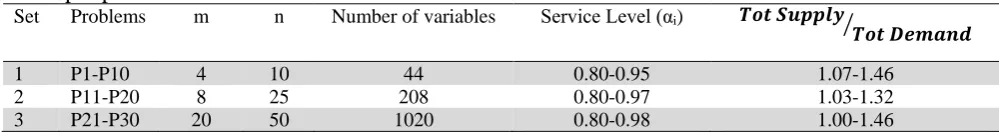
Three sets of different problems (10 problems per each set), each with different sizes and properties have been randomly generated to evaluate performance of proposed hybrid algorithm. The performance measure compares results of applying hybrid algorithm with optimal solution. Table 1 summarizes size, number of variables, service level of facilities and ratio between the total supply and the total demand for each set. This ratio depends on the demand distribution of customers and service level of facilities. Thus,
Tot supply/Tot demand that is reported in Table 1 is obtained after determining demands and service levels for each problem. Service levels are generated uniformly in the interval [0.8,1.0].
Table 1
The input parameters
Set Problems m n Number of variables Service Level (αi) 𝑻𝑻𝑻𝑻𝑻𝑻𝑺𝑺𝑺𝑺𝑺𝑺𝑺𝑺𝑺𝑺𝑺𝑺
𝑻𝑻𝑻𝑻𝑻𝑻𝑫𝑫𝑫𝑫𝑫𝑫𝑫𝑫𝑫𝑫𝑫𝑫 �
1 P1-P10 4 10 44 0.80-0.95 1.07-1.46
2 P11-P20 8 25 208 0.80-0.97 1.03-1.32
3 P21-P30 20 50 1020 0.80-0.98 1.00-1.46
The coordinates of facilities and demand points locations in set 1 are generated as U(0,100), U(0,200), U(0,300), U(0,400) and U(0,600). In set 2 coordinates are obtained from U(0,200), U(0,300), U(0,400) U(0,500) and U(0,1000) and in set 3 coordinates are generated as U(0,650), U(0,1000), U(0,1200), U(0,1500) and U(0,2000). ( U(a,b) is uniform distribution in interval [a,b] ). In the following, dispersion of candidate facilities and demand points in each problem is shown on 30 different scatter charts. The square markers in the charts represent location of candidate facilities, while the circle markers show the location of customers. Serving costs are generated as set 1 , part of set 3 and set 4 of test problems in Holmberg et al. (1999). They are determined as 𝑐𝑐𝑖𝑖𝑖𝑖 = 𝑥𝑥𝑐𝑐𝑖𝑖𝑖𝑖 where 𝑐𝑐𝑖𝑖𝑖𝑖 is Euclidean distance between facility 𝑐𝑐 and customer 𝑗𝑗 and 𝑥𝑥 is a positive scalar. Customer demands generated from a uniform distribution in ranges [1,5] and [1,6]. We have tested various settings for fixed costs and amount of orders that each facility can serve. Fixed costs range from 100 to 1000 in set 1. In set 2 fixed costs range from 300 to 10000 and in set 3 from 1800 to 30000. Amount of orders served by facilities is generated as
𝑈𝑈([1 ×𝑦𝑦×104], [5 ×𝑦𝑦×104]) when customer demand ranges in 𝑈𝑈(1,5) and as 𝑈𝑈 ��1 ×𝑦𝑦×10
4�, [6 ×𝑦𝑦× 10
4]� when customer demand is generated in 𝑈𝑈(1,6). [𝑥𝑥] represents the greatest integer less or equal to 𝑥𝑥 and 𝑦𝑦 is a scalar equals to 1.1 , 1.2, 1.3 or 1.4.
The Tests
Table 2
The results of hybrid algorithm values versus optimal values
Problem Optimal value Hybrid algorithm value Gap
P1 1319 1319 0.0000
P2 2213 2213 0.0000
P3 4143 4143 0.0000
P4 3592 3592 0.0000
P5 4506 4506 0.0000
P6 6184 6184 0.0000
P7 1238 1248 0.0080
P8 1620 1620 0.0000
P9 2805 2805 0.0000
P10 3787 3787 0.0000
P11 5055 5055 0.0000
P12 53256 53298 0.0008
P13 62885 63000 0.0018
P14 9749 9807 0.0059
P15 61963 62241 0.0045
P16 50341 50381 0.0008
P17 37031 37184 0.0041
P18 48133 48133 0.0000
P19 39937 39937 0.0000
P20 23736 23791 0.0023
P21 77292 77695 0.0052
P22 81501 82233 0.0090
P23 480088 481796 0.0035
P24 68132 68132 0.0000
P25 38445 38732 0.0075
P26 72977 73127 0.0021
P27 173891 174447 0.0032
P28 26408 26540 0.0050
P29 68255 68827 0.0084
P30 60076 60609 0.0087
The analysis of the computational results obtained by the hybrid algorithm, testifies the efficiency of proposed methodology for solving problems. The maximum gap, in all instances, between optimal objective function value and the value obtained by our hybrid algorithm is 0.9% and the average gap is 0.27%. In Table 3, maximum, minimum and average gap in different sets is presented.
Table 3
The summary of max/min and average gap
Set Problem Max Gap Min Gap Average Gap
1 P1-P10 0.0080 0.0000 0.0008
2 P11-P20 0.0059 0.0000 0.0020
3 P21-P30 0.0090 0.0000 0.0053
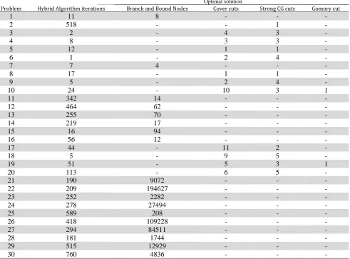
Table 4
The results of hybrid algorithm iterations, branch and bound nodes, and number of cuts
Optimal solution
Problem Hybrid Algorithm iterations Branch and Bound Nodes Cover cuts Strong CG cuts Gomory cut
1 11 8 - - -
2 518 - - 1 -
3 2 - 4 3 -
4 8 - 3 3 -
5 12 - 1 1 -
6 1 - 2 4 -
7 7 4 - - -
8 17 - 1 1 -
9 5 - 2 4 -
10 24 - 10 3 1
11 342 14 - - -
12 464 62 - - -
13 255 70 - - -
14 219 17 - - -
15 16 94 - - -
16 56 12 - - -
17 44 - 11 2 -
18 5 - 9 5 -
19 51 - 5 3 1
20 113 - 6 5 -
21 190 9072 - - -
22 209 194627 - - -
23 252 2282 - - -
24 278 27494 - - -
25 589 208 - - -
26 418 109228 - - -
27 294 84511 - - -
28 181 1744 - - -
29 515 12929 - - -
30 760 4836 - - -
6. Conclusions
Stochastic capacitated facility location problem with single sourcing is formulated and a hybrid algorithm is presented to solve it efficiently. Set of potential capacitated facilities is to be selected to serve customers with uncertain demand while facilities fixed costs and costs of shipments are minimized. Each customer must be served only with one facility as the model is single sourcing. The power of proposed algorithm is embedded in its heuristic nature which is capable of solving SSSCFLP problems efficiently. The hybrid algorithm consists of a Lagrangian heuristic coupled to an adjusted mixture of ant colony and genetic meta-heuristics. The Lagrangian relaxation is solved by solving a number of knapsack problems and the Lagrangian dual is solved by subgradient optimization. The computational results lead to the following conclusions: The Lagrangian relaxation together with subgradient optimization provide strong lower bounds to the problem. The adjusted mixture of ant colony and genetic optimization is very powerful in finding optimal or near optimal solutions.
References
Neebe, A. W., & Rao, M. R. (1983). An algorithm for the fixed-charge assigning users to sources
problem. Journal of the Operational Research Society, 34, 1107-1113.
Ahuja, R. K., Orlin, J. B., Pallottino, S., Scaparra, M. P., & Scutellà, M. G. (2004). A multi-exchange
heuristic for the single-source capacitated facility location problem. Management Science, 50(6),
749-760.
Barceló, J., & Casanovas, J. (1984). A heuristic Lagrangean algorithm for the capacitated plant location
problem. European Journal of Operational Research,15(2), 212-226.
Beasley, J. E. (1993). Lagrangean heuristics for location problems. European Journal of Operational
Research, 65(3), 383-399.
Chen, C. H., & Ting, C. J. (2008). Combining lagrangian heuristic and ant colony system to solve the
single source capacitated facility location problem.Transportation research part E: logistics and
transportation review, 44(6), 1099-1122.
Cortinhal, M. J., & Captivo, M. E. (2003). Upper and lower bounds for the single source capacitated
location problem. European journal of operational research,151(2), 333-351.
Holmberg, K., Rönnqvist, M., & Yuan, D. (1999). An exact algorithm for the capacitated facility location
problems with single sourcing. European Journal of Operational Research, 113(3), 544-559.
Hindi, K. S., & Pieńkosz, K. (1999). Efficient solution of large scale, single-source, capacitated plant
location problems. Journal of the operational Research Society, 50(3), 268-274.
Tragantalerngsak, S., Holt, J., & Rönnqvist, M. (2000). An exact method for the two-echelon,
single-source, capacitated facility location problem. European Journal of Operational Research, 123(3),
473-489.
Klincewicz, J. G., & Luss, H. (1986). A Lagrangian relaxation heuristic for capacitated facility location
with single-source constraints. Journal of the Operational Research Society, 37(5), 495-500.
Lin, C. K. Y. (2009). Stochastic single-source capacitated facility location model with service level