R E S E A R C H A R T I C L E
Open Access
Surveillance of dengue vectors using
spatio-temporal Bayesian modeling
Ana Carolina C. Costa
1,2*, Cláudia T. Codeço
3, Nildimar A. Honório
4,5, Gláucio R. Pereira
5,
Carmen Fátima N. Pinheiro
5and Aline A. Nobre
3Abstract
Background: At present, dengue control focuses on reducing the density of the primary vector for the disease, Aedes aegypti, which is the only vulnerable link in the chain of transmission. The use of new approaches for dengue entomological surveillance is extremely important, since present methods are inefficient. With this in mind, the
present study seeks to analyze the spatio-temporal dynamics ofA. aegyptiinfestation with oviposition traps, using
efficient computational methods. These methods will allow for the implementation of the proposed model and methodology into surveillance and monitoring systems.
Methods: The study area includes a region in the municipality of Rio de Janeiro, characterized by high population density, precarious domicile construction, and a general lack of infrastructure around it. Two hundred and forty traps
were distributed in eight different sentinel areas, in order to continually monitor immatureAedes aegyptiandAedes
albopictusmosquitoes. Collections were done weekly between November 2010 and August 2012. The relationship between egg number and climate and environmental variables was considered and evaluated through Bayesian zero-inflated spatio-temporal models. Parametric inference was performed using the Integrated Nested Laplace Approximation (INLA) method.
Results: Infestation indexes indicated that ovipositing occurred during the entirety of the study period. The distance between each trap and the nearest boundary of the study area, minimum temperature and accumulated rainfall were all significantly related to the number of eggs present in the traps. Adjusting for the interaction between temperature and rainfall led to a more informative surveillance model, as such thresholds offer empirical information about the favorable climatic conditions for vector reproduction. Data were characterized by moderate time (0.29 – 0.43) and spatial (21.23 – 34.19 m) dependencies. The models also identified spatial patterns consistent with human population density in all sentinel areas. The results suggest the need for weekly surveillance in the study area, using traps allocated between 18 and 24 m, in order to understand the dengue vector dynamics.
Conclusions: Aedes aegypti, due to it short generation time and strong response to climate triggers, tend to show an eruptive dynamics that is difficult to predict and understand through just temporal or spatial models. The proposed methodology allowed for the rapid and efficient implementation of spatio-temporal models that considered zero-inflation and the interaction between climate variables and patterns in oviposition, in such a way that the final model parameters contribute to the identification of priority areas for entomological surveillance.
Keywords: Entomological surveillance, Dengue, Bayesian methods, Spatio-temporal models, Zero-inflated models, INLA
*Correspondence: [email protected]
1Sergio Arouca National School of Public Health, Oswaldo Cruz Foundation, Rua Leopoldo Bulhões 1.480, Rio de Janeiro, Brazil
2National Institute of Women, Children and Adolescents Health Fernandes Figueira, Department of Clinical Research Oswaldo Cruz Foundation, Avenida Rui Barbosa 716, Rio de Janeiro, Brazil
Full list of author information is available at the end of the article
Background
The complexity of dengue transmission has motivated the development of many studies to assess the numerous fac-tors related to the circulation and persistence of this dis-ease in human populations. While significant progress has been made, numerous questions remain unanswered, and an effective dengue control plan is still an open problem. No effective vaccines or antiviral drugs are currently avail-able, impeding a direct intervention on the human link in the dengue transmission cycle. As such, current con-trol measures are still focused on reducing the vectorial capacity ofAedes aegypti.
The Household Infestation index (HI) and the Breteau index (BI) are the standard mosquito abundance measure-ments used to evaluate the effectiveness of vector control strategies [1]. However, these indices, based on the sur-vey of breeding sites with mosquito larvae, are poorly correlated with the abundance of the adult mosquito population, which is directly responsible for the disease transmission [2]. For example, a study has shown high dengue incidence when HI was below 3 % in Salvador city, Northeastern Brazil [3].
Ovitrap has been proposed as an alternative tool for Aedes aegypti monitoring in areas with low mosquito abundance [4]. This trap was created by Fay and Eliason [5] and perfected by Reiter and Gubler [6], and provides measures of ovipositing activity. Although not a direct measure of mosquito abundance, studies have shown a strong correlation between egg count and the density of the female mosquito population [7].
Despite the advantages of trapping over larval surveys, this approach is still scarcely applied to surveillance. One of the main reasons for this is the fact that the sampling and statistical properties of the measurements produced are not entirely understood yet. In this study, data from a long-term surveillance program carried out under very controlled conditions in eight sentinel areas, provide an opportunity to develop and test innovative models and contribute to the development of an analytical frame-work to be implemented inAedes aegyptimonitoring sys-tems. The models proposed are computationally intensive and more efficient methods that allow for their imple-mentation in surveillance and monitoring systems were investigated. Such information contributes to the develop-ment ofAedescontrol activities focused on areas and time periods affected by the most severe mosquito infestations.
Methods
Study area
The study area is the Manguinhos campus of the Oswaldo Cruz Foundation (Fiocruz), located in the city of Rio de Janeiro, Brazil (22°52’30”S, 43°14’53”W; 697.000m2). The area surrounding the campus is characterized by densely populated urban zones, precarious living conditions and
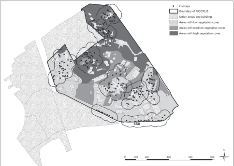
a general lack of infrastructure [8]. Eight sentinel areas were identified for continuous monitoring of immature Aedes aegyptiandAedes albopictus, each one representing different degrees of forest cover, distances to neighbour-ing residential areas, and intensity of human commutation and permanence. Sentinel Areas (SA) were designated as SA1–SA8 (Fig. 1). Table 1 describes the area and the vegetation-type percentage for each SA.
Entomological monitoring
Thirty ovitraps were randomly placed in each SA with a minimum distance of 20 m between traps. Traps consisted of black plastic pots containing water, hay infusion and a eucatex paddle. Egg collections occurred weekly from November 2010 to August 2012, for a total of 89 uninter-rupted weeks. The collected material was transported to the Sentinel Operational Unit of Mosquito Vectors (NOS-MOVE/Fiocruz). Each paddle was carefully inspected for egg positivity and, when confirmed, the number of eggs was quantified. The sampling using ovitraps is part of the project “Monitoring of populations ofAedes aegypti on the Fiocruz campus” which is coordinated by Dr. Honório and was approved by the Vice-Presidency of Environment, Healthcare and Health Promotion (VPAAPS) of Fiocruz.
Climate and environmental variables
Maximum and minimum temperatures were collected from the São Cristóvão meteorological station, located at a 3 km-distance from the study area, while accumulated rainfall was extracted from the Penha station, roughly 5 km away (source: Sistema Alerta Rio website [9], oper-ated by the city of Rio de Janeiro).
To delimit the area of each SA, 50 m-radius influence zones were created for each trap, based its geographical location, using ArcGis 10.0 software. In order to calcu-late the percent green cover for each of the eight areas, a campus map was intersected with the oviposition traps by vectorizing a high-resolution satellite image. Finally, the distance between each trap and the nearest boundary of the study area was calculated and is hereby referred to as Border Distance.
Spatio-temporal modeling
Fig. 1Map of Manguinhos campus at Oswaldo Cruz Foundation. Characterization of green space, and localization of oviposition traps in eight sentinel areas (SA). The SAs were located at different altitudes, in such a way that none of the habitats overlapped
processes are occurring: presence of eggs is driven by the mosquito choice of the ovitrap for ovipositing, and the abundance of eggs is driven by the number of females that chose the ovitrap. This can be formalized as following:
fZAP(y;ζ,μ)=
1−ζ y=0
ζ ×fZAP(y;μ) y>0,
in which 1−ζrepresents the probability of the absence of oviposition. Analogously,ζis the probability of the occur-rence of oviposition and will be referred to as positivity.
Let the random variable Y(si,t) represents the num-ber of eggs in trap i, i = 1,. . ., 30 at week t, for t = 1,. . ., 89. Moreover, let y(si,t) be the realization of the spatio-temporal processY(si,t), when oviposition occurs.
Table 1Descriptors
Sentinel Area Area Vegetation type (%)
(SA) (m2) Urban Low Medium Dense Total
SA1 42,701.18 8 0 16 59 83
SA2 41,388.24 35 0 5 61 100
SA3 46,051.25 26 0 10 64 100
SA4 57,714.65 36 51 0 5 92
SA5 43,686.54 25 53 18 4 100
SA6 43,515.28 28 47 25 0 100
SA7 61,048.08 24 26 50 0 100
SA8 71,055.57 18 53 0 0 71
A
v
er
age density of eggs
Dec−10 Jan−11 Feb−11 Mar−11 Apr−11 Ma
y−11
J
un−11 Jul−11 Aug−11
Sep−11 Oct−11 No
v−11
Dec−11 Jan−12 Feb−12 Mar−12 Apr−12 Ma
y−12
J
un−12 Jul−12 Aug−12
0
100
200
300
400
500 Area (% of zeros)
SA1 (30%) SA2 (24%) SA3 (35%) SA4 (32%) SA5 (45%) SA6 (33%) SA7 (35%) SA8 (58%)
(a)
Rainfall (lag 2) (mm)
Dec−10 Jan−11 Feb−11 Mar−11 Apr−11 Ma
y−11
J
un−11 Jul−11 Aug−11
Sep−11 Oct−11 No
v−11
Dec−11 Jan−12 Feb−12 Mar−12 Apr−12 Ma
y−12
J
un−12 Jul−12 Aug−12
0 20 40 60 80 100 120 140 14 16 18 20 22 24 26 28 Minim um temper
ature (lag 1) (ºC)
Rainfall (lag 2) Minimum temperature (lag 1)
(b)
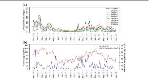
Fig. 2Temporal Series. Time series of the average weekly egg density and the zero-egg collection week frequency in each of the eight SAs (a), accumulated rainfall (lag 2) and minimum temperature (lag 1) (b)
It is assumed thaty(si,t)has a ZAP distribution with an average ofμ(si,t)and the following equations:
y(si,t)|y(si,t) >0 ∼ ZAP(μ(si,t)) (1) log(μ(si,t)) = z(si,t)β+ξ(si,t)+ε(si,t), (2) ξ(si,t) = aξ(si,t−1)+ω(si,t) (3)
fort > 1, wherez(si,t) = (z1(si,t),. . .,zp(si,t))denotes the vector of pcovariates for trapiin time t, and β =
β1,. . .,βp
is the vector of coefficients representing their effects. Additionally, ε(si,t) ∼ N
0,σε2 is the mea-surement error defined by a Gaussian white noise, both serially and spatially uncorrelated. In the geostatistics lit-erature, the termz(si,t)βis referred to as the large-scale component – in this case depending on meteorological and environmental covariates – while the varianceσε2is called the nugget effect [11]. Finally,ξ(si,t)is a space-time Gaussian Field (GF) that follows an auto-regressive first-order dynamics, with temporal correlation coefficient a and evolution error given by ω(si,t), in which |a| < 1 and ξ(si, 1) derived from the stationary distribution N0,σω2/(1−a2). Additionally, ω(si,t) has a Gaussian distribution with zero average, no time dependence and characterized by the following covariance function
Cov(ω(si,t),ω(sj,t))=
0 ift=t
σ2
ωC(h) ift=t,
fori = j. The spatial correlation functionC(h) depends on the spatial Euclidean distance between locationssiand
sj, such thath= || si−sj || ∈R. This way, the process is assumed to be second-order stationary and isotropic [11]. It follows immediately thatVar(ω(si,t))=σω2, for eachsi andt. The spatial correlation functionC(h)is defined by the Matérn covariance function
C(h)= 1
(ν)2ν−1(κh)νKν(κh), (4) withKνdenoting the modified Bessel function of the sec-ond type and order ν > 0. The parameter ν, which is usually kept fixed, measures the smoothness of the pro-cess. In other words,νcontrols the behavior of the covari-ance function for measures that are separated by small distances. On the other hand,κ >0 is a scaling parameter related to rangeρ, i.e., a distance at which spatial correla-tion becomes small. In particular, we use the empirically derived definitionρ =
√
8ν
κ , withρcorresponding to the distance at which spatial correlation is approximately 0.1, for eachν(see Lindgren et al. [12] for further details).
tested for interaction with every other climate variable in the model. Figure 2b shows the climate variables compos-ing the model. Besides the aforementioned variables, the only environmental covariate considered for inclusion in the spatio-temporal model was border distance. Because the variable-measuring scales were different, each covari-ate was standardized by subtracting the mean and dividing it by the standard deviation.
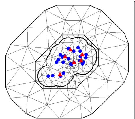
We used 24 traps for model fitting (blue dots in Fig. 3) and the remaining six traps to validate the model (red triangles in Fig. 3). The predictive performance of the models was evaluated by calculating the percentage of observations, which fell within the 95 % credibility inter-vals for validating data.
In addition to the adjustment of individual models per SA, a hierarchical model was also considered for the whole set of sentinel areas.
Hierarchical model
This model is similar to the one presented above, but includes an area-specific random effect. In this analysis, from the total of 240 traps, 192 traps were used for model fitting and 48 ones for validation. As before, the effect of the interaction among climate variables was also tested. The validity of the model was checked as before.
SPDE approach
ξ is a spatially structured GF pursuant to the effect of ω, in such a way that it can be considered to be a mul-tivariate Normal distribution.˜ is the dense correlation matrix, which describes the covariance structure ofξ. The
Fig. 3Triangulation. Locations of the 30 oviposition traps in the sentinel area 1 (SA1) and triangulation of SA1 with 147 vertices. Blue circles identify the traps used to estimate model parameters and red triangles identify those used for validation of the proposed model
factorization of˜ has a computational cost of the order O(n3), which can pose a problem in case of large array. Thus, the suggestion is to represent the GF as a Gaussian Markov Random Field (GMRF) based on Stochastic Par-tial DifferenPar-tial Equations (SPDE) [15].
The GMRF is a process that models the spatial depen-dence of the data by areal unit, such as regular/irregular grids, or by geographic region. The primary advantage of using GMRF instead of GF entails its strong computa-tional properties. The computacomputa-tional advantage of making inference with GMRF stems directly from the sparsity of the precision matrix , so that linear algebra oper-˜ ations can be performed using numerical methods for sparse matrices, resulting in a substantial computational gain [16].
The objective of the SPDE approach is in the way it iden-tifies the GMRF, with local neighborhood and a sparse precision matrix, which best describes the Matérn field – a GF with a Matérn covariance function. Given this rep-resentation, it is possible to derive inference from the GMRF through the use of its good computational proper-ties. Essentially, the SPDE approach uses a finite element representation to define the Matérn field as a linear com-bination of base functions defined on a triangulation of the domainD. This consists of subdividingDinto a set of triangles that do not intersect and have maximum one edge or vertex in common [15]. Figure 3 illustrates the concept of triangulation in SA1.
Integrated nested Laplace approximation (INLA)
Letθ =ζ,β,σε2,a,σω2,κdenote the parameter vector to be estimated. The joint posterior distribution is given by:
π(θ,ξ,μ|y)∝π(y|μ)π(μ|ξ,θ)π(ξ|θ)π(θ) (5) whereπ(·)denotes the probability density function,y =
{yt}, μ = {μt} andξ = {ξt} with t = 1,. . .,T. Usu-ally, independent prior distributions are chosen for the parameters, so thatπ(θ) = dim(i=1θ)π(θi). Considering that conditionally on μ the observations yt are serially independent and that the state process follows Markovian time dynamics, the Eq. (5) can be written as:
π(θ,ξ,μ|y) ∝
T
t=1
π(yt|μt) T
t=1
π(μt|ξt,θ)
×
π(ξ1|θ) T
t=2
π(ξt|ξt−1,θ)
π(θ)
Approximation (INLA) method, proposed by Rue et al. [18], as an alternative to MCMC methods. The main advantage of INLA over MCMC is computational, as the algorithm rapidly produces accurate approximations to posterior marginals distributions for the latent variables, as well as for the hyperparameters.
Unlike the MCMC, where posterior inference is based on simulations, the INLA method directly ties distribu-tions of interest with a closed form expression. Therefore, the convergence diagnosis inherent to MCMC methods is not a problem. The main objective of the INLA approach is to approximate the posterior marginal distributions of the latent field and of the hyperparameters, given by:
π(ξi|y) =
π(ξi|θ,y)π(θ|y)dθ (6)
π(θj|y) =
π(θ|y)dθ−j. (7)
This approach is based on an efficient combination of Laplace approximations for the full conditional distribu-tions π(θ|y) andπ(ξi|θ,y), i = 1,. . .,n, and numerical integration routines to integrate out the hyperparameters θ.
The INLA method as proposed in Rue et al. (2009) includes three main approximation steps to obtain the marginal posteriors in (6) and (7). The first step entails approximating the full posteriorπ(θ|y). Firstly, it is nec-essary to obtain an approximation of the full conditional distribution ofξ,π(ξ|y,θ), using a multivariate Gaussian density πG(ξ|y,θ) (see Rue and Held [16] for further details) and evaluate it in your mode. Then, the pos-terior density of θ is approximated using the Laplace approximation
π(θ|y)∝ π(ξ,θ,y)
πG(ξ|θ,y)
ξ=ξ∗(θ),
where ξ∗(θ) is the mode of the full conditional ofξ for a given θ. Since there is no exact closed form forξ∗(θ), an optimization scheme is necessary. Rue et al. [18] cal-culated this mode using the Newton-Raphson algorithm. The posteriorπ(θ|y) will be used later to integrate out the uncertainty with respect toθwhen approximating the posterior marginal ofξi.
The second step involves calculating the Laplace approximation of the full conditionalsπξi|y,θfor some values of θ. These values will be used as evaluation points in the numerical integration to obtain the poste-rior marginals ofξiin (6). The distribution ofπ(ξi|θ,y)is approximated using the Laplace approximation defined by
πLA
ξi|θ,y
∝ π
ξ,θ,y
πG
ξ−i|ξi,θ,y
ξ−i=ξ−∗i(ξi,θ), (8)
where ξ−i is the vector ξ with the i-th component omitted, πG
ξ−i|ξi,θ,y
is the Gaussian approximation
of πξ−i|ξi,θ,y
, considering ξi as fixed (observed) and ξ∗−i(ξi,θ)is the mode ofπ
ξ−i|ξi,θ,y
. The approximation ofπξi|θ,y
using (8) can be expen-sive, sinceπG
ξ−i|ξi,θ,y
have to be recalculated for each value ofξi andθ. Rue et al. [18] proposed two cheaper alternatives to obtain these distributions. The first one is the Gaussian approximationπG
ξi|θ,y
, which provides reasonable results in a short computational time; how-ever, according to Rue and Martino [19], its accuracy can be affected by several factors. These problems can be corrected with moderate computational cost using a sim-plified version of the Laplace approximation, defined as the series expansion ofπLA
ξi|θ,y
aroundξi = μi(θ), the mean ofπGξi|y,θ[18].
At last, the full posteriors obtained through the two pre-vious steps are combined and the marginal densities of ξi andθjare obtained by integrating the irrelevant terms. The approximation for the marginal of the latent variables can be obtained by
πξi|y
=
πξi|y,θ
πθ|ydθ
≈
k
πξi|θk,y
πθk|y
k,
(9)
which is evaluated on a set of grid pointsθkwith weights k, fork=1, 2,. . .,K. According to Rue et al. [18], since the integration points are selected in a regular grid, it is feasible to assume all the weightsk to be equal. A sim-ilar numerical integration procedure is used to evaluate the marginalsπθj|y
. Since the dimension ofθ is small (less than or equal to seven), these numerical routines are effective in returning a discretized representation of the marginal posteriors.
A good choice of the setθkof evaluation points is impor-tant for the accuracy of the above numerical integration s teps. Rue et al. [18] suggest to compute the negative Hessian matrix S at the modeθ∗, ofπθ|yand to consider its spectral value decomposition,S−1 = QQT. Then,θ is defined through a standardized variablez, such that:
z=QT−1/2θ−θ∗ or θ(z)=θ∗+Q1/2z
and a collectionZ ofz values is obtained, such that the correspondingθ(z) points are located around the mode θ∗. Starting fromz =0 (θ =θ∗), each component entry
ofzis searched in the positive and negative directions in step sizes ofηz. Allzpoints that satisfy
logπθ(0)|y−logπθ(z)|y< ηπ
are considered to be belonging toZ. The set of evaluation points is based on the values inZ. An appropriate calibra-tion of ηzandηπ values must be performed, in order to produce accurate approximations.
using the R software version 3.0.1 [20] in the R-INLA package [21].
Results
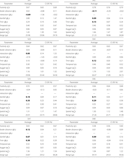
Summaries of the posterior means of the model’s fixed effects and their respective 95 % credibility intervals (CI) are shown in Table 2. The “interaction” component, whenever shown, represents the effect of the interaction between accumulated rainfall in the two weeks prior to collection and the minimum temperature in the week prior to collection on the number of eggs. In the pres-ence of statistically significant interaction, the primary effects of variables involved in the interaction terms are not interpreted, in order to avoid erroneous conclusions. All the models fit the data reasonably well, with 58 to 88 % of the validation dataset encompassed by the 95 % CI. The validation analysis could capture the oviposition pattern for all SAs, except for the highest number of eggs. Additional file 1 shows the validation analysis per trap for one particular SA (SA6).
The positivity index ranged from 0.38 to 0.78. The area with the least positivity was SA8, and the most “attractive” for oviposition was SA2. Border distance had significant effect on the reduction of the number of eggs in SA2, and contributed to an increase in eggs in SA7. Total accu-mulated rainfall (Rainfall) was important to explain the increase in the number of eggs in all SAs except SA4. Min-imum temperature (Tmin) also significantly contributed to explain the egg frequency in all SAs, except SA8.
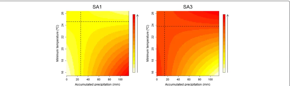
Interaction effects between climate variables in SA1 and SA3 suggest that the effect of the quantity of accumulated rainfall (lag 2) on egg abundance changes as a function of the minimum temperature (lag 1). Figure 4 shows how the interaction between these variables influenced egg den-sity, highlighting the change in direction of the effects for values above or below 26.3 mm of rain and 24.6 °C mini-mum temperature in SA1. In this area, an increase in the number of eggs could be expected only if the total rain-fall was more than 26.3 mm, and minimum temperatures fell below 24.6 °C. In SA3, the effects changed direction according to the thresholds of 14.5 mm and 23.8 °C, so that rainfall greater than 14.5 mm and temperatures below 23.8 °C favored a reduction in egg density.
The temporal correlation between the weekly average number of eggs was moderate, varying from 0.29 (SA8) to 0.46 (SA2 and SA4). The variance of the nugget effect or measurement error ranged from 0.02 (SA7) to 0.09 (SA5 and SA8). The posterior mean of the spatial effect vari-ance ranged from 1.04 (SA8) to 1.79 (SA4). More variation is explained by the spatial term rather than by the mea-surement error in all SAs. The empirical range varied from 21.23 to 34.19 m (the maximum distance between traps was 182.6 and 623.8 m) occurring respectively in SA2 and SA8. As these are the distances at which correlation
is close to 0.1, we can conclude that the data feature moderate spatial correlation, which slowly decreases with distance.
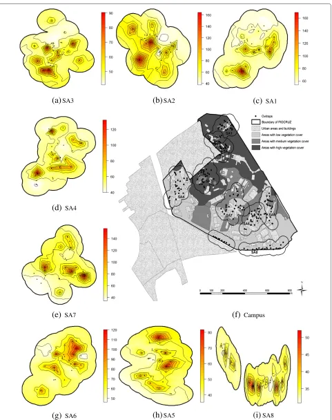
The mean spatial egg distribution during the study period is presented in Fig. 5. In each area, the filled cir-cle indicates the traps’ location. In general, the highest concentration of eggs was found in areas that bordered settlements with high population densities (slums), and in those close to campus buildings, where pedestrian foot traffic was heavier. Within each area, egg distribution was heterogeneous. Additional file 2 shows weekly changes in the number of eggs in SA1 throughout the study period using an animated map.
The hierarchical model estimated an average positivity of 62.2 %. Border distance was not important to explain the variations in the number of eggs, so it did not enter in the final model. The accumulated rainfall in the two weeks prior to trap installation was statistically significant but the minimum temperature in the previous week was not, as well as the interaction between them. As expected, higher rain rates (β2 = 0.08 [95 % CI: 0.01 − 0.16]) was associated with larger quantities of eggs. The variabil-ity attributed to the spatial-structured effect (σω2 = 8.98 [95 % CI: 6.98−12.42]) was greater than that attributed to measurement error (σε2=0.17 [95 %CI: 0.15−0.19]), while the temporal correlation (a) found was 0.77 (0.71 -0.83). The variance attributable to the random effect was 0.02 (0.02 - 0.03), suggesting homogeneity among SAs. The estimated empirical range (ρ = 37.27 [95 % CI: 32.25−42.13]) suggests that the results from the hierar-chical model are similar to those of individual models. The validation dataset encompassed by the 95 % CI was 57.8 %.
Discussion
Due to the complexity of estimation involved in spatio-temporal modeling, these dimensions of variation inher-ent to many epidemiological processes are rarely analyzed together. The present methodology for estimation allows for the rapid and efficient implementation of these models, while considering 1) zero-inflation within SA, 2) interaction among climate variables and 3) different oviposition patterns over the course of the study period. This methodology can contribute to the identification of priority areas for entomological surveillance and targeted fieldwork.
Oviposition activity occurred over the entire course of the study but varied among SAs. The highest ovitrap pos-itivity was 78 % (76–79 %) in SA2, while the lowest one was 38 % (36–38 %) in SA8. The remaining SAs pre-sented ovitrap positivities varying between 55 and 67 % (Table 2). As expected, summertime featured the greatest infestation.
Table 2Individual models
SA1 SA2
Parameter Average CI (95 %) Parameter Average CI (95 %)
Positivity(ζ ) 0.67 0.65 0.69 Positivity(ζ ) 0.78 0.76 0.79
Border distance(β1) 0.02 –0.08 0.11 Border distance(β1) –0.11 –0.20 –0.02
Interaction(β4) –0.69 –1.36 –0.02 Interaction(β4) — — —
Rainfall(β2) 0.80 0.13 1.47 Rainfall(β2) 0.09 0.04 0.14
Tmin(β3) 0.29 0.19 0.40 Tmin(β3) 0.15 0.07 0.24
Temporal(a) 0.40 0.32 0.47 Temporal(a) 0.46 0.38 0.52
Nugget(σ2
ε) 0.06 0.05 0.07 Nugget(σε2) 0.06 0.05 0.07
Spatial(σ2
ω) 1.45 1.30 1.62 Spatial(σω2) 1.66 1.47 1.87
Range(ρ) 25.98 23.06 29.76 Range(ρ) 21.23 18.06 24.04
SA3 SA4
Parameter Average CI (95 %) Parameter Average CI (95 %)
Positivity(ζ ) 0.64 0.62 0.67 Positivity(ζ ) 0.65 0.63 0.67
Border distance(β1) 0.03 –0.04 0.11 Border distance(β1) 0.03 –0.07 0.13
Interaction(β4) 0.85 0.14 1.55 Interaction(β4) — — —
Rainfall(β2) –0.74 –1.45 –0.03 Rainfall(β2) 0.00 –0.05 0.06
Tmin(β3) 0.10 –0.00 0.19 Tmin(β3) 0.12 0.03 0.21
Temporal(a) 0.30 0.21 0.42 Temporal(a) 0.46 0.40 0.52
Nugget(σε2) 0.08 0.05 0.10 Nugget(σε2) 0.04 0.03 0.05
Spatial(σ2
ω) 1.16 1.01 1.32 Spatial(σω2) 1.79 1.53 2.07
Range(ρ) 29.96 25.44 34.56 Range(ρ) 26.47 21.85 34.15
SA5 SA6
Parameter Average CI (95 %) Parameter Average CI (95 %)
Positivity(ζ ) 0.55 0.53 0.57 Positivity(ζ ) 0.66 0.64 0.68
Border distance(β1) –0.04 –0.13 0.05 Border distance(β1) –0.03 –0.11 0.06
Interaction(β4) — — — Interaction(β4) — — —
Rainfall(β2) 0.10 0.04 0.17 Rainfall(β2) 0.11 0.05 0.17
Tmin(β3) 0.35 0.25 0.44 Tmin(β3) 0.29 0.21 0.38
Temporal(a) 0.35 0.30 0.41 Temporal(a) 0.35 0.27 0.41
Nugget(σε2) 0.09 0.07 0.10 Nugget(σε2) 0.04 0.03 0.06
Spatial(σω2) 1.31 1.17 1.47 Spatial(σω2) 1.30 1.12 1.48
Range(ρ) 25.91 23.73 28.06 Range(ρ) 27.26 23.71 31.90
SA7 SA8
Parameter Average CI (95 %) Parameter Average CI (95 %)
Positivity(ζ ) 0.65 0.62 0.67 Positivity(ζ ) 0.38 0.36 0.40
Border distance(β1) 0.12 0.04 0.21 Border distance(β1) 0.01 –0.08 0.09
Interaction(β4) — — — Interaction(β4) — — —
Rainfall(β2) 0.07 0.01 0.14 Rainfall(β2) 0.09 0.02 0.16
Tmin(β3) 0.30 0.22 0.39 Tmin(β3) 0.06 –0.04 0.16
Temporal(a) 0.32 0.25 0.39 Temporal(a) 0.29 0.18 0.41
Nugget(σ2
ε) 0.02 0.01 0.05 Nugget(σε2) 0.09 0.05 0.12
Spatial(σ2
ω) 1.36 1.21 1.54 Spatial(σω2) 1.04 0.87 1.22
Fig. 4Interaction effects. Map of the interaction effects between total rainfall (lag 2) and minimum temperature (lag 1) on the average egg density in SA1 and SA3, according to changes in the total rainfall and minimum temperature. The quadrants formed by dashed black lines delimit the influence of climate variables on average egg density, according to the thresholds of 26.33 mm (total rainfall)/24.6 °C (minimum temperature) in SA1 and 14.5 mm (total rainfall)/23.8 °C (minimum temperature) in SA3. The ascending color scale indicates the range of values for egg density with respect to the total rainfall and minimum temperature values
mosquitoes came from outside the campus [8]. If this was true, significant negative effect would be found. How-ever, such result was only observed in SA2, which limits a densely populated slum. All the other SAs presented nonsignificant or inverted relationship (SA7). This oppo-site trend suggests that the eggs captured in SA7 are not from outside mosquitoes, but from mosquitoes estab-lished inside. Within the campus, the greatest egg collec-tion occurred in areas close to buildings and passages, in comparison to more isolated areas. Indeed, on the same campus, Honório et al. [8] found statistically sig-nificant relationship between the number of mosquito larvae in artificial breeding sites within the campus and the distance to the border in both the wet and dry sea-sons. The anthropophilic behavior ofAedes aegyptiis well documented.
A model containing the interaction between tempera-ture and rain was more informative and provides thresh-olds that could be used to issue alerts. However, the threshold values differed between areas, being significant only in two areas, SA1 and SA3 (Fig. 4). This varia-tion suggests local microclimate effects not captured by the single meteorological station and can be attributed to the particular characteristics of each area (Table 1). Minh An and Rocklöv [22] evaluated the effect of the interaction between rain and temperature on the num-ber of dengue cases in Hanoi, Vietnam. They showed rain occurrence and temperatures between 15 and 30 °C to correlate to an increase in the number of dengue cases.
Total precipitation accumulated over the two weeks prior to collection contributed to the increase in the num-ber of eggs in five of the SAs, located within both high and low levels of vegetation areas. SA1 and SA3 also fea-tured the effect of rain, but this effect interacted with
temperature. Only SA4 showed no association between the number of eggs and rainfall. The relationship between precipitation and the proliferation ofA. aegyptiis likely to vary on small geographical scales [23]. Rain contributes to the formation of breeding habitats, but this effect will depend on the local availability of containers [24]. During heavy rainfall, these water containers offer favorable con-ditions for oviposition and the development of immature mosquitoes.
2 A S
(b)
3A S
(a)
(c) SA1
(d) SA4
(e) SA7
(g) SA6
(h)
SA5(i)
SA8(f) Campus
The joint analysis of the sentinel areas (Hierarchical model) only confirmed the rainfall as driving the num-ber of eggs. Nevertheless, the estimates of spatial and temporal dependence parameters were similar.
The present study had some limitations. Other data, such as wind direction and speed were not available for analysis, as well as other potentially confounding variables, such as the amount and location of breeding sites. Moreover, precipitation data were collected from a weather station 5 km away from the study area. This may introduce bias, as the quantity of rainfall can vary substantially even in close geographical areas.
Aside from these limitations, the results suggest that border distance, minimum temperature and precipitation are all associated with population density ofA. aegypti. Maps describing the abundance of eggs identified areas with high potential for transmission, so that control and prevention activities could be developed. The results also indicates the ideal spacing for traps, which constitutes an important aspect of sampling.
Conclusions
Aedes aegypti, due to it short generation time and strong response to climate triggers, tend to show an erup-tive dynamics that is difficult to predict and understand through just temporal or spatial models. Spatio-temporal modeling has been prohibitive due the computational costs involved in MCMC based parameter estimation. Our results suggest that INLA based inference increases the efficiency of the estimation process in a way to allow its calculation within the time frame expected for any surveillance program. Differently from other ovitrap sur-veys, the studied dataset consisted of a high density of traps placed at close distances, and surveyed very fre-quently. This design allowed to assess the spatial and temporal autocorrelation structure of the oviposition pro-cess. The short range of these correlations support the notion that high sampling is necessary to capture the spatio-temporal patterns of mosquito activity, for exam-ple, the identification of hotspots. The extrapolation of these results to other areas must be done with care. Ideally, this study should be replicated in other settings. How-ever, despite the specific results obtained, we believe this framework (zero-inflation+ truncated Poisson model+ INLA based inference) is an efficient way to model ovipo-sition dynamics anywhere.
Additional files
Additional file 1: Validation analysis for SA6.Validation analysis per trap for SA6 throughout the study period. (PDF 23.6 Kb)
Additional file 2: Animated map for SA1.Animated map of weekly changes in the number of eggs in SA1 throughout the study period. This file can be viewed with: QuickTime Player. (MP4 11980 kb)
Abbreviations
BI: Breteau index; Bin: Binomial distribution; CI: Credibility intervals; DIC: Deviance information criterion; Fiocruz: Oswaldo Cruz foundation; GF: Gaussian field; GMRF: Gaussian Markov random field; HI: Household infestation index; ICICT: Institute of scientific and technological communication and information in health; INLA: Integrated nested Laplace approximation; MCMC: Markov chain Monte Carlo methods; NOSMOVE: Sentinel operational unit of mosquito vectors; Rainfall: Total accumulated rainfall; SA: Sentinel areas; SPDE: Stochastic partial differential equations; Tmin: Minimum temperature; VPAAPS: Vice-presidency of environment, healthcare and health promotion; ZAP: Zero-altered poisson distribution.
Competing interests
The authors declare that there is no conflict of interests.
Authors’ contributions
ACCC performed all analyses, interpreted results, and wrote the first and final drafts of the manuscript. AAN and CTC advised on the statistical analyses and the drafting of the manuscript. NAH performed the study design, coordinated the study and critically revised the manuscript. GRP and CFNP participated in the study design and were responsible for data collection and tabulation. All authors read and approved the final manuscript.
Acknowledgements
The authors would like to thank the Sentinel Operational Unit of Mosquito Vectors (NOSMOVE/Fiocruz) for data collection, processing and tabulation, as well as the technical team from the Geoprocessing Laboratory at the Health Institute of Scientific and Technological Communication and Information (ICICT) at the Oswaldo Cruz Foundation for generating the campus map, border distance and percent ground cover. This project was funded by the Dengue Fiocruz Network.
Author details
1Sergio Arouca National School of Public Health, Oswaldo Cruz Foundation, Rua Leopoldo Bulhões 1.480, Rio de Janeiro, Brazil.2National Institute of Women, Children and Adolescents Health Fernandes Figueira, Department of Clinical Research Oswaldo Cruz Foundation, Avenida Rui Barbosa 716, Rio de Janeiro, Brazil.3Scientific Computing Program, Oswaldo Cruz Foundation, Avenida Brasil 4365, Rio de Janeiro, Brazil.4Laboratory of Transmitters of Hematozoa, Oswaldo Cruz Institute, Oswaldo Cruz Foundation, Avenida Brasil 4365, Rio de Janeiro, Brazil.5Sentinel Operational Unit of Mosquito Vectors, Oswaldo Cruz Foundation, Avenida Brasil 4365, Rio de Janeiro, Brazil.
Received: 22 May 2015 Accepted: 3 November 2015
References
1. Ministério da Saúde. Secretaria de vigilância em Saúde. Diretoria Técnica de Gestão: Levantamento Rápido de índices Para Aedes Aegypti LIRAa -Para Vigilância Entomológica do Aedes Aegypti No Brasil: Metodologia Para Avaliação Dos índices de Breteau e Predial e Tipo de Recipientes. Brasil; 2013. Ministério da Saúde. Secretaria de vigilância em Saúde. Diretoria Técnica de Gestão.
2. Braga IA, Valle D. Aedes aegypti: vigilância, monitoramento da resistência e alternativas de controle no brasil. Epidemiologia e Serviços de Saúde. 2007;16(4):295–302.
3. Teixeira MG, Barreto ML, Costa MCN, Ferreira LDA, Vasconcelos PFC. Avaliação de impacto de ações de combate ao Aedes aegypti na cidade de Salvador, Bahia. Rev Bras Epidemiol. 2002;5:108–15.
4. Gomes AC. Medidas dos níveis de infestação urbana para aedes (stegomyia) aegypti e aedes (stegomyia) albopictus em programa de vigilância entomológica. Informativo Epidemiológico do SUS. 1998;5: 49–57.
5. Fay RW, Eliason DA. A preferred oviposition site as a surveillance method for aedes aegypti. Mosq News. 1966;26:531–5.
6. Westaway EG, Blok J. Taxonomy and evolutionary relationships of flaviviruses In: Gubler DJ, Kuno G, editors. Dengue and Dengue Hemorrhagic Fever. Wallingford, UK: CAB International; 1997. p. 147–174. 7. Codeço CT, Lima AWS, Araújo SC, Lima JBP, Maciel-de-Freitas R,
index with four alternative traps. PLoS Neglected Tropical Diseases. 2015;9(2):e0003475. Public Library of Science.
8. Honório NA, Castro MG, Barros FS, Magalhães MA, Sabroza PC. The spatial distribution of Aedes aegypti and Aedes albopictus in a transition zone, Rio de Janeiro, Brazil. Cad Saude Publica. 2008;25(6):1203–14. 9. Sistema Alerta Rio. http://alertario.rio.rj.gov.br/.
10. Zuur AF. Zero Inflated Models and Generalized Linear Mixed Models with R. United Kingdom: Highland Statistics Limited; 2012.
11. Cressie NAC. Statistics for Spatial Data. Revised Edition. Hoboken, NJ, USA: John Wiley & Sons, Inc; 1993.
12. Lindgren F, Rue H, Lindström J. An explicit link between gaussian fields and gaussian markov random fields: the stochastic partial differential equation approach. J R Stat Soc Ser B (Stat Methodol). 2011;73(4):423–98. 13. Spiegelhalter DJ, Best NG, Carlin BP, Van Der Linde A. Bayesian measures
of model complexity and fit. J R Stat Soc Ser B (Stat Methodol). 2002;64(4): 583–639. doi:10.1111/1467-9868.00353.
14. How Are the Deviance Information Criteria (DIC) and The
Watanabe-Akaike Information Criterion (WAIC) computed? http://www.r- inla.org/faq#TOC-How-are-the-Devicance-Information-Criteria-DIC-and-The-Watanabe-Akaike-information-criterion-WAIC-computed-/. 15. Cameletti M, Lindgren F, Simpson D, Rue H. Spatio-temporal modeling
of particulate matter concentration through the spde approach. Adv Stat Anal. 2013;97(2):109–31.
16. Rue H, Held L, Vol. 104. Gaussian Markov Random Fields: Theory and Applications. Monographs on Statistics and Applied Probability. London: Chapman & Hall; 2005.
17. Gamerman D, Lopes HF. Monte Carlo Markov Chain: Stochastic Simulation for Bayesian Inference. London, UK: Chapman & Hall; 2006. 18. Rue H, Martino S, Chopin N. Approximate bayesian inference for latent
gaussian models by using integrated nested laplace approximations. J R Stat Soc Ser B (Stat Methodol). 2009;71(2):319–92.
19. Rue H, Martino S. Approximate Bayesian inference for hierarchical Gaussian Markov random field models. Journal of Statistical Planning and Inference. 2007;137(10):3177–3192.
20. R Core Team. R: A Language and Environment for Statistical Computing. Vienna, Austria: R Foundation for Statistical Computing; 2013. Foundation for Statistical Computing, http://www.R-project.org/.
21. Rue H, Martino S. INLA: Functions Which Allow to Perform a Full Bayesian Analysis of Structured Additive Models Using Integrated Nested Laplace Approximation. 2009. http://www.r-inla.org/.
22. Minh An DT, Rocklöv J. Epidemiology of dengue fever in hanoi from 2002 to 2010 and its meteorological determinants. Global Health Action. 2014;7:23074.
23. Halstead SB. Dengue virus - mosquito interactions. Annu Rev Entomol. 2008;53:273–91.
24. Alto BW, Juliano SA. Precipitation and temperature effects on populations of aedes albopictus (diptera: Culicidae): implications for range expansion. J Med Entomol. 2001;38(5):646–56.
25. Focks DA, Haile DG, Daniels E, Mount GA. Dynamic life table model for aedes aegypti (diptera: Culicidae): simulation results and validation. J Med Entomol. 1993;30:1018–28.
26. Jansen CC, Beebe NW. The dengue vector aedes aegypti: what comes next. Microbes Infect. 2010;12:272–9.
27. Honório NA, Codeço CT, Alves FC, Magalhães MA, Lourenço-D-Oliveira R. Temporal distribution of aedes aegypti in different districts of rio de janeiro, brazil, measured by two types of traps. J Med Entomol. 2009;46(5): 1001–1014.
28. Duncombe J, Clements A, Davis J, Hu W, Weinstein P, Ritchie S. Spatiotemporal patterns of aedes aegypti populations in cairns, Australia: assessing drivers of dengue transmission. Tropical Med Int Health. 2013;18(7):839–49.
29. Padmanabha H, Durham D, Correa F, Diuk-Wasser M, Galvani A. The interactive roles of aedes aegypti super-production and human density in dengue transmission. PLoS Negl Trop Dis. 2012;6(8):1799.
Submit your next manuscript to BioMed Central and take full advantage of:
• Convenient online submission
• Thorough peer review
• No space constraints or color figure charges
• Immediate publication on acceptance
• Inclusion in PubMed, CAS, Scopus and Google Scholar
• Research which is freely available for redistribution