A Web-Based Sample Size Calculator for Reliability Studies

(1)

67 Education in Medicine Journal. 2018; 10(3): 67–76

www.eduimed.com  Penerbit Universiti Sains Malaysia. 2018

RESOURCES

A Web-based Sample Size Calculator for

Reliability Studies

Wan Nor Arifin

Unit of Biostatistics and Research Methodology, School of Medical Sciences, Universiti Sains Malaysia, Kelantan, MALAYSIA

To cite this article: Wan Nor Arifin. A web-based sample size calculator for reliability studies.

Education in Medicine Journal. 2018;10(3):67–76. https://doi.org/10.21315/eimj2018.10.3.8

To link to this article: https://doi.org/10.21315/eimj2018.10.3.8

ABSTRACT

Planning a validation study of a questionnaire or measurement tool requires consideration for testing the validity and reliability aspects of the measurement tool. When it comes to the reliability aspect, a number of commonly used statistical coefficients such as Cronbach’s alpha, intraclass correlation, kappa and Pearson’s correlation coefficients would be considered to provide empirical evidence of the reliability of the tool during the validation process. To ensure that the reliability is accurately assessed, a researcher must consider the sample size requirement for the statistical analyses. In this article, I will introduce a newly developed web-based sample size calculator, which includes the ability to calculate the sample sizes of these four important coefficients. I will also show how to use the calculator for each of the coefficients.

Keywords: Reliability study, Sample size calculator, Web-based

INTRODUCTION

Planning a validation study of a questionnaire or measurement tool requires taking into account the validity and reliability aspects of the measurement tool. For the reliability aspect, a number of commonly used statistical coefficients such as Cronbach’s alpha, intra-class correlation (ICC), kappa and Pearson’s correlation coefficients will be considered to provide empirical evidence of the reliability of the measurement tool. At the same time, a researcher must consider the sample size requirement for the selected reliability coefficients in his study. This is important to ensure that the planned study will have a sufficient sample size for accurate assessment of reliability.

Sample size calculation is not easy. The researcher must formulate proper study objectives, the approach to the inferential statistics and only then he should select suitable sample size calculation methods for the selected statistical analyses (1). For simple sample size calculations, such as for single mean and proportion, the formulas are quite simple, thus can be easily calculated by hand (provided he knows the right formulas). However, most will rely on sample size calculators available as personal computer software, phone applications or web-based calculators. Personally, I would suggest using sample size calculators instead of plugging in values in the sample size formulas because it is easy to commit mistakes while doing the calculation by hand.

Volume 10 Issue 3 2018

DOI: 10.21315/eimj2018.10.3.8

ARTICLE INFO

Submitted: 17-07-2018 Accepted: 14-08-2018 Online: 28-09-2018

CORRESPONDING AUTHOR _{Dr. Wan Nor Arifin, Unit of Biostatistics and Research Methodology, School of Medical}

(2)

Sample size calculators for reliability coefficients are relatively scarce. A good example of freely available web-based sample calculator for reliability coefficients is StatsToDo (2). Another example would be in form of a commercial software known as PASS (3). Given this scarcity, I initially developed a sample size calculator in the form of a spreadsheet (4), with the intention of making it easier for my undergraduate and postgraduate students to calculate sample sizes. As long as they have spreadsheet programmes in their computers, tablets or smart phones, they can use the spreadsheet to calculate the sample sizes.

Later, I found it difficult to navigate through the spreadsheet interface on phones, thus I started developing a web-based sample size calculator (5). I mainly focused the development for the reliability coefficients, while leaving the rest of

sample size formulas for future updates. The development was made possible with free web hosting on GitHub development platform (6), and JavaScript Statistical Library (7). The web-based calculator is accessible at https://wnarifin.github.io/ssc_ web.html (Figure 1).

In this article, I will introduce the newly developed web-based sample size calculator, which includes the ability to calculate the sample sizes for these four important coefficients. I will also show how to use the calculator for each of the coefficients. The web-based calculator allows flexibility while using the calculator because its use is not restricted to any specific operating systems. It does not require installation of the software or any additional software to start using it. A working Internet connection and a web browser is all it needs to use the calculator.

(3)

CRONBACH’S ALPHA

Background

Cronbach’s alpha coefficient indicates the internal consistency reliability of a set of items in a factor. It ranges between 0 (not reliable at all) to 1 (perfect reliability, theoretically speaking). However, in practice

it should not exceed 0.9 (8), otherwise the items are redundant or repetitive.

About the Calculator

The calculator is accessible at https:// wnarifin.github.io/ssc/ssalpha.html. The interface of the calculator is shown in Figure 2.

(4)

Two methods to calculate the sample size for Cronbach’s alpha coefficient are available in the calculator. The first method is the hypothesis testing method. The calculator uses the formula given by Bonett (9). The form consists of the minimum acceptable Cronbach’s alpha (H0, null

hypothesis), expected Cronbach’s alpha (H1,

alternative hypothesis), significance level (α), statistical power (1–β), number of items (k), and expected dropout rate. By default, the minimum acceptable Cronbach’s alpha is set as 0.65, which corresponds to the minimally acceptable value of the coefficient (10). The expected Cronbach’s alpha is what a researcher expects to get in his study. This can be based on his experience, expert opinion or previous studies. The significance level (α) in this calculator is programmed for a two-tailed hypothesis test and the default is α = 0.05. This is set as such for the sake of standardisation in the interface design of the calculator, because in many situations sample size calculation is done for a two-tailed test. For a one-two-tailed hypothesis test, multiply the desired α by two. For example, for a one-tailed test with α = 0.05, α is set as 0.05 × 2 = 0.10 in the calculator. The number of items refers the number of items in a domain or factor. Please keep in mind not to set the number as the number of items for the whole questionnaire, but the number of items in a specific domain. If there are three factors proposed for a concept in a questionnaire, with five, seven and ten items respectively, calculate the sample size required for each factor and take the largest of the calculated sample sizes. The expected dropout rate increases the calculated sample size so as to take into account the possible dropouts and invalid cases in the study. The formula for this adjustment follows the one given in (1).

The second method is the estimation method which also utilises the formula given by Bonett (9). The form consists of the expected Cronbach’s alpha, precision,

confidence level, number of items (k), and expected dropout rate. Again, the expected Cronbach’s alpha here is based on a researcher’s experience, expert opinion or previous studies. The confidence level follows the commonly used level of 95% confidence interval estimation. The precision here is related to the confidence interval that a researcher expects to get during the analysis. For example, he expects the Cronbach’s alpha will be 0.85, with a 95% confidence interval of 0.75 to 0.95. Here, the precision is plus-minus the expected Cronbach’s alpha (the point estimate), which is 0.85 ± 0.10 (0.75– 0.85 = −0.10, 0.95–0.85 = 0.10). The number of items and expected dropout rate were explained above.

Example 1

A factor consisting of 10 items is expected to have a Cronbach’s alpha = 0.8, with the minimum acceptable value of the coefficient is 0.7. A significance level α = 0.05 for a one-tailed test (because we want to test against the null hypothesis of ≥ 0.7) and a power of 80% are specified. Remember to multiply 0.05 by two for the one-tailed α. The dropout rate is expected = 20%.

Sample size, n = 86 subjects.

Sample size (with 20% dropout), n_drop = 108 subjects.

Example 2

A factor consisting of 10 items is expected to have a Cronbach’s alpha = 0.8 ± 0.1 the precision and a confidence level of 95%. The dropout rate is expected = 20%.

(5)

INTRACLASS CORRELATION (ICC)

Background

Intraclass correlation coefficient indicates the degree of agreement between repeated measurements of a numerical variable. The coefficient ranges from −1 (poor agreement) to 1 (perfect agreement). The coefficient is used to indicate the agreement between

raters (inter-rater reliability), consistency of raters on repeated occasions (intra-rater reliability), and test-retest reliability.

About the Calculator

The calculator is accessible at https://

wnarifin.github.io/ssc/ssicc.html. The interface of the calculator is shown in Figure 3.

(6)

Two methods to calculate the sample size for ICC coefficient are available in the calculator. The first one is the hypothesis testing method, using the formula given by Walter, Eliasziw and Donner (11). The form consists of the minimum acceptable ICC (ρ0), expected ICC (ρ1), significance level

(α), statistical power (1–β), number of raters or repetitions per subject (k), and expected dropout rate. By default, the minimum acceptable ICC is set as 0.6, which is the cutoff value for the good ICC (12). The expected ICC is the ICC that a researcher expects to get in his study, which is based on his experience, expert opinion or literature review. The number of raters per subject is the number of raters involved in interrater reliability assessment, while the number of repetitions refers to the number of times a rater repeats his assessment (intrarater reliability) or how many times test-retest sessions are done. The rest of the options were already explained before.

The second one is the estimation method which uses the formula given by Bonett (13). The form consists of the expected ICC, precision, confidence level, number of raters or repetitions (k), and expected dropout rate. The expected ICC and precision are decided by the researcher. The rest of the options were similar to that of Cronbach’s alpha.

Example 3

The test-retest reliability of a measurement tool by ICC is expected = 0.85. The measurement was taken at two occasions (two repetitions). The lowest acceptable ICC is 0.7. A significance level α = 0.05 for a one-tailed test (remember to set α = 0.1) and a power of 80%. The dropout rate is expected = 10%.

Example 4

The interrater reliability of the manual blood pressure measurement using mercury sphygmomanometer is expected to be high with ICC = 0.9. Five medical doctors (the raters) are involved. The precision is 0.05 with a confidence level of 95%. The dropout rate is expected = 10%.

KAPPA

Background

Kappa coefficient indicates the degree of agreement between raters on a categorical variable (nominal or ordinal). The coefficient ranges from −1 (poor agreement) to 1 (perfect agreement). Similar to ICC, the coefficient is used to indicate the agreement between raters (interrater reliability), consistency of raters on repeated occasions (intrarater reliability) and test-retest reliability.

About the Calculator

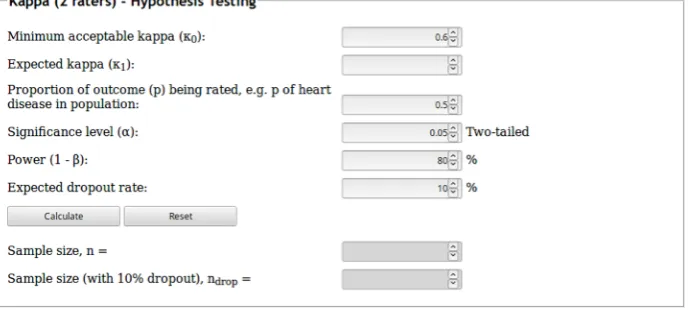
The calculator is accessible at https:// wnarifin.github.io/ssc/sskappa.html. The interface of the calculator is shown in Figure 4.

(7)

(although it might be implemented in the future). Interested readers may try using

kappaSize package in R software (15) for the

estimation method.

The form consists of the minimum acceptable kappa (κ0), expected ICC (κ1),

proportion of outcome (p) being rated, significance level (α), statistical power (1–β), and expected dropout rate. By default, the minimum acceptable kappa is set as 0.6, which is considered as substantial by Landis and Koch (16). The expected kappa is the expected kappa value in a reliability study, which indicates the extend of agreement between two raters. The p of outcome is the proportion of the rated outcome in the target population, for example the outcome being rated is the presence of pulmonary tuberculosis based on chest X-ray films of patients with prolonged cough and the

proportion of pulmonary tuberculosis among patients with prolonged cough is known to be around 0.75 (75%). The rest of the options were already explained in the preceding sections.

Example 5

Two radiologists are studied for their agreement on rating of X-ray films for the presence of pneumonia. It is known that the presence of pneumonia among patients with shortness of breath is 30% (p = 0.3). The minimum acceptable kappa is 0.6. The expected kappa is 0.9 at a significance level of α = 0.05 (one-tailed), power of 80%. The dropout rate is expected = 30%.

(8)

PEARSON’S CORRELATION

Background

Pearson’s correlation coefficient indicates the strength of linear relationship between two numerical variables. The coefficient ranges from −1 (perfect negative correlation) to +1 (perfect positive correlation). The coefficient is commonly used to indicate the convergence between factors in a

psychometric tool and the relationship between a tool with another comparison tool. It is also used to indicate the test-retest reliability, although using ICC in this case is preferable.

About the Calculator

The calculator is accessible at https:// wnarifin.github.io/ssc/sscorr.html. The interface of the calculator is shown in Figure 5.

(9)

There are two methods implemented in the calculator to calculate the sample size for Pearson’s correlation coefficient. The first method is the hypothesis testing method. The calculator uses the formula given in (17). The form consists of the expected correlation (r), significance level (α), statistical power (1–β), and expected dropout rate. The rest of the options were explained previously in the Cronbach’s alpha section. By default, the expected correlation is set as 0.3, which is the medium effect size according to Cohen (18). The second one is the estimation method. The formula used (Equation 8) is given in (19). The form consists of the expected correlation (r), precision, confidence level, and expected dropout rate. Again, the expected correlation here is set as 0.3 for the medium Cohen’s effect size, while the rest of the options were similar to that of Cronbach’s alpha and ICC.

Example 6

A researcher expects a positive correlation between body mass index (BMI) and cholesterol level (one-tailed test because the correlation is expected in one direction, i.e. positive). The strength of correlation is expected at r = 0.4. A one-tailed significance level α = 0.05 (i.e. 0.1 in the calculator) and a power of 90% are specified. The dropout rate = 20%.

Example 7

A researcher expects a correlation between the depression domain in a newly developed ABC inventory and the depression domain in Depression Anxiety Stress Scales (DASS). He is unsure whether the association will negative of positive (two-tailed test because the correlation is expected in either direction, i.e. positive and negative). The strength of correlation is expected at r = 0.4. A two-tailed significance

level α = 0.05 and a power of 90% are specified. The dropout rate = 20%.

Example 7

A researcher expects a correlation between the depression domain in a newly developed ABC inventory and the depression domain in DASS. The strength of correlation is expected at r = 0.5 ± 0.1 the precision and a confidence level of 95%. The dropout rate = 20%.

CONCLUSION

In this article I introduced the newly developed web-based sample size calculator with the ability to calculate the sample sizes for Cronbach’s alpha, ICC, kappa, and Pearson’s correlation coefficients. I also showed how to use the calculator, especially on the choice of the minimum acceptable values, expected values, and precision, and how to change the significance level

α for one-tailed tests. With a working Internet connection and a web browser, any researchers can easily calculate the required sample sizes for most common coefficients in reliability analysis. I hope researchers in medical education and other fields of sciences will find the calculator useful in planning their research and calculate the sample sizes for their research proposals.

REFERENCES

(10)

2. Chang A, Sahota, D. StatsToDo [Internet]. 2014 [cited 11 July 2018]. Available from: https://www.statstodo.com/index.php

3. NCSS statistical software [Internet]. PASS 16 Power Analysis and Sample Size Software. 2018. Available from: https://ncss. com/software/pass.

4. Arifin WN. Sample size calculator (Version 2.0) [Spreadsheet file]. Author; 2017. Available from: http://wnarifin.github.io

5. Arifin WN. Sample size calculator (web) [Internet]. 2018 [cited 11 July 2018]. Available from: http://wnarifin.github.io 6. GitHub, Inc. Github [Internet]. USA:

GitHub, Inc.; 2018 [cited 11 July 2018]. Available from: https://github.com/

7. Norris T. JavaScript Statistical Library (jStat) [Internet]. USA: GitHub Inc. 2018 [cited 11 July 2018]. Available from: http://jstat.github.io/

8. Streiner DL. Starting at the beginning: an introduction to coefficient alpha and internal consistency. J Pers Assess. 2003;80(1):99–103. https://doi.org/10.1207/ S15327752JPA8001_18

9. Bonett DG. Sample size requirements for testing and estimating coefficient alpha. Journal of Educational and Behavioral Statistics. 2002;27(4):335–40. https://doi. org/10.3102/10769986027004335

10. DeVellis RF. Scale development: theory and applications. California: Sage Publications; 2012.

11. Walter SD, Eliasziw M, Donner A. Sample size and optimal designs for reliability studies. Stat Med. 1998;17(1):101–10. https://doi.org/10.1002/(SICI)1097-0258 (19980115)17:1<101::AID-SIM727>3.0. CO;2-E

12. Cicchetti DV. Guidelines, criteria, and rules of thumb for evaluating normed and standardized assessment instruments in psychology. Psychological Assessment. 1994;6(4):284–290. https://doi.org/10.1037/ 1040-3590.6.4.284

13. Bonett DG. Sample size requirements for estimating intraclass correlations with desired precision. Stat Med. 2002;21(9):1331–5. https://doi.org/10.1002/ sim.1108

14. Donner A, Eliasziw M. A goodness-of-fit approach to inference procedures for the kappa statistic: confidence interval construction, significance-testing and sample size estimation. Stat Med. 1992;11:1511–9. https://doi.org/10.1002/sim.4780111109 15. Rotondi MA. kappaSize: sample size

estimation functions for studies of interobserver agreement [R package]. Author; 2013. Available from: https:// CRAN.R-project.org/package=kappaSize 16. Landis JR, Koch GG. The measurement

of observer agreement for categorical data. Biometrics. 1977;33(1):159–74. https://doi. org/10.2307/2529310

17. Machin D, Campbell MJ, Tan SB, Tan SH. Sample size tables for clinical studies. 3rd ed. West Sussex, UK: John Wiley & Sons Ltd; 2009.

18. Cohen J. A power primer. Psychol Bull. 1992;112(1):155–9. https://doi.org/10.1037/ 0033-2909.112.1.155