Defining an Elasticity Metric for Cloud Computing
Environments
Marta Beltrán
Department of Computing, ETSII Universidad Rey Juan Carlos
28933 Madrid, Spain
[email protected]
ABSTRACT
Elasticity is a key property of cloud computing environments and one of the features which distinguishes this paradigm from other ones. An elasticity metric could be used to de-fine and to monitor Service Level Agreements (SLAs), to compare and to benchmark different cloud providers or to improve provisioning and management decisions in real time if it could be measured with some simple procedure, to men-tion only some examples. Unfortunately, there are not still standard elasticity metrics capable of easily capturing its main components or aspects, these are, scalability, accuracy, time and cost. This work defines a new elasticity metric for cloud computing environments which not only captures these four essential components but also provides a simple procedure to analyse elasticity in cloud contexts. The ob-tained experimental results on a real cloud environment ev-idence that this new elasticity metric is able to quantify the degree of elasticity obtained in different cloud scenarios and to establish interesting comparisons and analysis.
Categories and Subject Descriptors
C.4 [Performance of Systems]: Performance attributes
General Terms
Experimentation, Performance
Keywords
Cloud Computing, Elasticity, Performance evaluation
1.
INTRODUCTION
Almost all definitions of cloud computing include features such as on-demand self-service, ubiquitous and heteroge-neous access, resource pooling and multi-tenancy, measured service and billing, dynamism or elasticity. These important properties of the paradigm offer businesses and individuals the possibility to access to infinite resources (cloud archi-tectures provide the illusion of infinite computing resources) from anywhere in the world, eliminating traditional capac-ity predictions, in-house confinement and long term commit-ments.
The on-demand feature allows users to adapt the system capacity to their requirements, scaling up or down the provi-sioned resources as the workload increases or decreases. The elasticity of a cloud system is related to this feature, refer-ring to the capability of adapting the leased capacity to the user’s requirements as exactly, fast and cheap as possible. Therefore, there are four main components that should be considered to define an elasticity metric: scalability, accu-racy, time and cost. Scalability, at least to certain degrees, is something guaranteed in almost all current cloud services. But it is usual that a cloud user is not able to scale exactly to the needed capacity at all times, for example, because the provider only offers certain types of service instances in her catalogue that makes impossible a perfect match. It is also usual that the scaling of resources needed to adapt to work-load changes involves a non-negligible delay. And finally, it has to be considered that capacity scaling may involve costs that make them not worthwhile in certain situations. As a result, most of cloud users do not pay for what they exactly need.
Although all current cloud services claim to be elastic, a plethora of factors affect their elasticity and there is not a simple and easy to understand and to measure metric to quantify this performance figure. The main contribution of this work is the definition and validation of a new elasticity metric for cloud environments. More specifically we (a) anal-yse the elasticity concept in cloud environments, discussing the most important factors affecting it and determining its main components (b) define a new elasticity metric for cloud services keeping it simple (c) describe a simple and stan-dard procedure to analyse this elasticity (d) validate the pro-posed metric and procedure with experiments performed on real cloud systems offering different services (e) identify the main elasticity enablers observed during the performed ex-periments. These contributions allow providers and users to have a complete characterization of their systems behaviour from a elasticity point of view and to optimize their designs,
VALUETOOLS 2015, December 14-16, Berlin, Germany Copyright © 2016 ICST
developments and deployments considering this important property, often mentioned so far, but very rarely quantified and used due to its usual complexity.
The rest of this paper is organized as follows. Section 2 analyses and discusses the elasticity concept, the related background and its implications in cloud environments. The new elasticity metric and the procedure proposed to analyse it are defined and described in Sections 3 and 4 respectively. Section 5 shows the most important experimental results obtained to validate the new metric in real scenarios and discusses some important observations. And finally Section 6 summarizes the conclusions of this work and the most interesting lines for future research.
2.
BACKGROUND ON ELASTICITY
Some cloud computing definitions make particular empha-sis on the importance of elasticity as a basic property of the paradigm, in fact, elasticity definitions emerged together with the cloud paradigm. But these works do not define elasticity metrics to quantify this essential property. In [17] a simple elasticity model is proposed: ifD(t) is the resource demand function andR(t) is the provisioned resources func-tion, perfect elasticity is achieved whenD(t) =R(t)∀t. This model assigns a cost to the situations in whichD(t)> R(t) (under-provisioning) and to the opposite situations in which
D(t) < R(t) (over-provisioning) and tries to quantify the total cost caused by not having a perfect elasticity.
This approach has been improved later in [10], using more sophisticated models and data obtained with real workloads executing on public clouds to assign costs to under-provisioning and over-provisioning situations. This new model consid-ers a penalty for provisioning resources that are not really needed but also for releasing resources that may be needed again soon. The figure of merit defined to perform compar-isons of elasticity among different cloud services is related to these penalties. In [3] an elasticity model is proposed too, in this case in order to understand the elasticity require-ments of a given application and if the elasticity provided by a cloud provider is able to meet those requirements. This work is focused on evaluating and comparing IaaS providers. On one hand, these definitions and models do not provide a general elasticity metric definition, but they all identify the aforementioned components (scalability, accuracy, time and cost), quantifying, considering and weighting them in different ways. On the other hand, some works have tried to define specific elasticity metrics. In [13] elasticity is defined as the degree a cloud layer autonomously adapts capacity to workload over time. This work presents a systematic lit-erature review of definitions and metrics for elasticity, but this is not the scope of our research. Anyway, some signif-icant examples are introduced in the following paragraphs because they were proposed with a ”keep-it-simple” philoso-phy similar to the one considered in our research.
In [14] the elasticity is considered an economic aspect of a cloud service besides cost. Elasticity is defined as the capability of both adding and removing resources rapidly in a fine-grain manner. In other words, an elastic cloud service concerns both growth and reduction of workload, and particularly emphasizes the speed of response to changed workload. Due to this essential relationship with the speed, the metrics proposed to quantify elasticity are the Provision (or Deployment) Time and the Boot Time (these two times as components of the Total Acquisition Time) as well as the
Suspend Time and the Delete Time (as components of the Total Release Time). Therefore, elasticity is quantified in time units, from 0 to∞.
In [5] authors claim that cloud users need to know whether a reduced load leads to a reduced bill. They propose to mea-sure elasticity by running a varying workload and comparing the resulting price with the price for the full load. In this case elasticity is measured in monetary units, going from 0 to∞.
In [8] elasticity is defined as the degree to which a system is able to adapt to workload changes by provisioning and de-provisioning resources in an autonomic manner, such that at each time the available resources match the current demand as closely as possible. Again accuracy and time are con-sidered. Being θthe average time to switch from a system configuration to another andµbe the average percentage of under-provisioned resources during the scaling process, the elasticity (El) is defined as:
El= 1
θ·µ (1)
Elasticity is in this case a metric measured intime units−1 from 0 to ∞. This definition has been also used in [9] to evaluate and to benchmark cloud elasticity.
Finally, in [1] an elasticity metric is supposed to answer these two questions: how often does the system violate its requirements? and once these requirements are violated, how long does it take before the system recovers to a state in which requirements are met again? In this work two metrics are defined to answer these questions, the number of SLO (Service Level Objectives) violations per time unit (from 0 to ∞) and the Mean Time To Quality Repair or MTTQR (in time units, from 0 to∞).
As it can be seen, although elasticity definitions and mod-els use to consider that scalability, accuracy, time and cost are its essential components, the previously defined elasticity metrics use to focus almost completely on time or cost as-pects. The elasticity quantified with these available metrics is usually completed with scalability, accuracy, efficiency, time or cost measurements and information in order to make evaluations, comparisons or decisions. As a result, current cloud users and providers need to handle complex sets of performance metrics when they are interested in elasticity.
In fact, there are multiple challenges related to defining a general elasticity metric in this context. First, no assump-tions about the cloud infrastructure, about the provision-ing and management mechanisms or about the application should be made. Second, the elasticity measurement has to be kept simple in order to avoid overheads and signifi-cant costs when it has to be performed frequently. Third, the four aforementioned components should be considered in a unique metric: scalability, accuracy, time and cost. And fourth, all the aspects affecting a service elasticity [6] should be determined and analysed to capture them in a proper way with the proposed metric, we will call them elasticity enablers the rest of this paper.
3.
DEFINITION OF A NEW ELASTICITY
METRIC
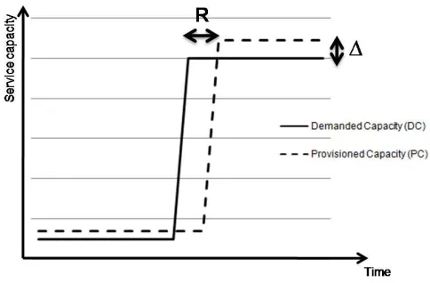
Figure 1: Inaccuracy (∆) and reconfiguration time (R) concepts
scale responding to the user needs fulfilling the QoS com-mitted in the SLA with optimum accuracy, speed and cost. And this elasticity of a cloud service should be quantified as:
E=f(scalability, accuracy, time, cost) (2)
Let us rely on a scalability metricψcapable of consider-ing cost in its definition. Figure 1 illustrates the definition of the service inaccuracy ∆ and of the service reconfiguration time R considered in this work, being the inaccuracy the absolute value of the difference between the exact capacity needed by the cloud user (demanded capacity orDC) and the actual provisioned capacity (provisioned capacity orP C) and the reconfiguration time the provisioning delay, there-fore, the time needed to reconfigure the service responding to the user’s needs. Notice that ∆ =|P C−DC|, with ab-solute value, because the service inaccuracy may cause an over-provisioning or an under-provisioning situation.
The higher the scalability value is, the higher must be the service elasticity; while the higher the ∆ andRvalues are, the lower must be the service elasticity. Therefore, trying to keep a simple definition, the elasticity metric could be:
E=ψ·g(1/∆)·h(1/R) (3) In this work the following definition is proposed:
E=
ψ·Rmin
R if∆ = 0
ψ·∆min
∆ ·
Rmin
R otherwise
(4)
Where,ψis the service scalability with a definition of scal-ability able to consider cost, ∆ is service inaccuracy, ∆minis
the minimum service inaccuracy,Ris the service reconfigu-ration time andRminis the minimum service reconfiguration time.
The minimum service inaccuracy (∆min) and minimum
service reconfiguration time (Rmin) are needed to quan-tify elasticity. In the first case, this minimum inaccuracy depends on the service granularity allowed by the service provider. Even relying on perfect elasticity mechanisms (mainly management and provisioning mechanisms), this
granularity may avoid a perfect match between demanded capacity and provisioned capacity. In the best case,g(∆)=1 because elasticity mechanisms achieve the minimum inaccu-racy. Otherwise,g(∆)<1 because the observed inaccuracy is greater than ∆min. A special case has to be considered to
avoid dividing by zero: the case in which ∆=0. This situa-tion is very unlikely, it only happens if full personalizasitua-tion of instances, containers, machine images, etc. is allowed and if perfect elasticity mechanisms are available. In this case we have always the perfect situation for elasticity andg(∆)=1. Regarding reconfiguration time, similar reasoning can be applied. The value forRmincan be specified by the provider in the SLA, can be computed from other times (resource ac-quisition time metrics such as provision time, boot time, startup time, spin up time, etc.) or it can be obtained with historic data. In this case, the function h(R) is defined as the ratio between the minimum reconfiguration time and the actual reconfiguration time. In the best case, h(R)=1 because elasticity mechanisms achieve the minimum recon-figuration time. Otherwise, h(R)<1 because the observed reconfiguration time is greater than Rmin. There are not special cases because there are not instantaneous reconfig-urations (even using proactive techniques, reconfiguring the service always involves a non-negligible latency) and the re-configuration time is always greater than zero.
With the provided definition, in the best caseE=ψ be-cause the accuracy and the reconfiguration times are the best possible (g(∆) = 1 and h(R) = 1). But this would not be a perfect elasticity case, because a minimum inac-curacy and/or a minimum reconfiguration time are always considered. Remember that the scalability is a necessary condition for elasticity, but not sufficient. To associate a meaning to the numerical value of elasticity, the scalability metric selection must be considered.
3.1
Discussing the scalability metric selection
Rather than having a definition of scalability which is uni-versally accepted, it is possible to find a number of scalability models that have been proposed during the last years. The main difference between all these models is in the selection of the performance metric used to characterize the system’s behaviour. Intuitively, a parallel or distributed system is scalable if its performance continues improving as the system size is increased. But, how this performance is quantified? A variety of metrics have been proposed: speedup [7, 15], efficiency [12], latency [18], power [11], average speed [16]. Other important differences are if they take into account or not the cost, how the system size is considered, and if they are able to support or not heterogeneous environments.In this research the P-scalability definition provided in [11], based on the power performance metric, has been cho-sen to quantify the scalability inside the elasticity definition due to a number of reasons:
• It takes into consideration the service cost, very im-portant for the elasticity definition.
• This metric can be used in homogeneous and hetero-geneous contexts.
• And finally, the strategy considered for scaling up the system is not only based on adding more processors or computing power, it can be much more complex considering another system resources and scaling paths (i.e. ways to increase the system size).
In [11], the scalability from configuration 1 to configura-tion 2 is defined as:
ψ=
P2 C2 P1 C1
(5)
In our case, P is the service power and C is the service cost (usually quantified as a cost per time unit). Therefore, with the P-scalability definition a service is scalable from configuration 1 to configuration 2 if the additional cost in-troduced by the service scaling is worthwhile considering the power gain.
The service cost of the target service configuration, C2 must always include the cost of the reconfiguration process. Therefore, it is not only the cost of the leased resources with configuration 2 but also of the scaling process needed to change the service from configuration 1 to configuration 2. This total cost should be divided byR, the reconfiguration time or provisioning delay, therefore, the time needed to reconfigure the service responding to the user’s needs. With this ratio, the cost per time unit can be computed.
C1= cost of the service per time unit in
the initial configuration 1 (6)
C2 = cost of the service per time unit in
the target configuration 2 + reconfiguration cost / R (7)
To consider the billing model in the new elasticity metric, financial measurements of this cost should be used. Re-member that provisioned resources are not always equal to charged resources, therefore, the typical cost metrics based on the quantity of provisioned or used resources do not al-ways capture the real cost of a service configuration. On the other hand the power definitionPselected for the scalability metric in this work is:
P =λ·f QoS, QoS
(8)
Where λ is the service admission throughput (accepted service requests per time unit),QoSis the observed quality of service quantified with the metric chosen by the user and the provider in the committed SLA andQoSis the expected or desired quality of service. It has to be pointed that this last value is not a mathematical expectation or average; it is a constant specified by the service user.
A typical example of theQoSmetric is the average appli-cation response time (T) for software as a service. The most simple functionf in cloud environments is:
f T, T
= T
T (9)
With this definition, the service power is high when its admission throughput is high and when theT value is close to its expected value,T.
But suppose that the user is running a parallel application on a HPC as a service context. In this case, the QoS may be the efficiency (ε). A differentf needs to be used, since a high response time value and a high efficiency value have opposite effects on the power figure. This function for the efficiency could be:
f(ε, ε) = ε
ε (10)
The two showed quality of service figures andf functions are very simple and very frequently used, but if another measure of this quality is needed in any context or a newf
function have to be defined by the service user to compute the system power with equation 8, it would be immediate to compute elasticity with these modifications.
4.
ELASTICITY ANALYSIS PROCEDURE
The elasticity quantification has a number of applications and it can be taken into consideration by cloud users and providers to define and to monitor the SLA or to make punc-tual provisioning decisions, for example. But another key idea in describing services elasticity is to perform an anal-ysis on a complete service scaling path controlled by a se-lected scaling factor (i.e. the aspect which is being modified to increase the system size) from a reference configuration rather on taking into account only the elasticity between two configurations. As it has been mentioned before, with the P-scalability the scaling factor is completely general. There-fore a deep analysis of all the aspects affecting the elasticity of a service could be performed. This analysis may be very useful, for example, in a provider selection context. But also in service design, development or deployment stages.First of all, a benchmark must be selected to perform the service analysis. This benchmark should include workloads that are representative of the user patterns of load variation and scaling (although for generic elasticity evaluations, sinu-soidal workloads, exponentially bursting workloads, linearly growing workloads or random workloads could be used, [10]). The typical scaling paths for cloud services are: increasing the number of provisioned instances, increasing the size of provisioned instances or increasing the number of users per application instance, the number of tasks per server image, etc.
At each scale factor the service can be optimally tuned (variable scaling strategy) by adjusting all its elasticity en-ablers, which are the parameters that can improve the ser-vice performance after its scaling, or it can be let unchanged (fixed scaling strategy). Then, the elasticity at this scale factor is computed comparing its value at this configuration with the elasticity of the reference case.
For example, if the selected scaling factor for the elastic-ity analysis is the number of provisioned instances, N, the proposed elasticity analysis should be performed following these steps:
1. Obtain the minimum and maximum configuration for the evaluated service estimating the minimum and the maximum number of instances (N0andNmax) allowed
2. Define the scaling strategy, from the reference case (N0) to the maximum service size (Nmax). The
fol-lowed scaling path can be:
• Fixed: When the scaling is performed only in-creasing the number of provisioned instances.
• Variable: When the scaling takes advantage of the elasticity enablers, tuning the service as best as possible for eachNvalue (for example, increas-ing the problem size, the grain size or adaptincreas-ing the load balancing and the virtual provisioning mechanisms as needed).
3. Select the quality of service metric interesting for the evaluated service, and define the correspondingf func-tion.
4. Obtain ∆minandRminfor all the consideredNvalues.
5. MeasureC,λ,QoS, ∆ andRfor all the consideredN
values.
6. Compute the elasticity for eachN value comparing it with the reference case,N0:
E(N0→N) =
ψ(N0→N)·RminR if∆ = 0
ψ(N0→N)·∆min∆ ·RminR otherwise
(11) With:
ψ(N0→N) =
PN CN PN0 CN0
(12)
5.
EXPERIMENTAL VALIDATION
In order to validate the new elasticity metric and the use-fulness of the procedure proposed to analyse it a private HPC-cloud has been used and two very different benchmarks at the application level have been selected. Specifically, we are interested in assessing the behaviour of the elasticity metric (reliability, repeatability, consistency, independence, etc.) and in verifying the utility of the proposed analysis procedure evaluating different elasticity enablers. Due to space restrictions only the most important and illustrative results will be summarized in this section.
5.1
Experimental setup
LazarusCloud is a private cloud providing IaaS, PaaS and SaaS for HPC applications. It is built with commodity hard-ware, 16 heterogeneous machines with Xen/Linux compose the cloud infrastructure. These 16 machines are connected by a Gigabit Ethernet network and a different server has been used during the experiments to emulate users and to generate all service requests.
In all the performed experiments two different scientific applications usually executed on LazarusCloud with three different problem sizes (class A, B and C from smaller to larger, 4X size increase going from one class to the next) have been selected as benchmarks for our experiments, a MonteCarlo simulation and a fluid physics simulation. The service request rate has been fixed in 5 requests per minute in our experiments for the two selected benchmarks, being this value set attending to the observations obtained from
real scenarios on LazarusCloud not detailed here for space restrictions.
LazarusCloud includes an additional machine used to run the AutoMAP mechanism proposed in [2]. AutoMAP (Au-tomatic Multi-tier Applications Provisioning) is a general (application and provider independent) application provi-sioning solution, it can be implemented with different archi-tectures from centralized to distributed and it is able to deal automatically with both batch and interactive applications allowing horizontal and vertical scaling (based on replication and on resizing respectively). As part of a research labora-tory one of the main goals of LazarusCloud is being able to avoid scientists the troubleshooting and decision-making related to service management, therefore the AutoMAP so-lution provides flexible and general mechanisms to automat-ically determine how much virtual resources need to be allo-cated to the application minimizing resources consumption and meeting the service level agreement. Only horizontal scaling has been used in our experiments.
For simplicity one instance type has been offered to end users to run their service requests based on a virtual machine with 2 virtual CPUs, 4 GB of memory and 80 GB of storage capacity. End users and the application cloud provider agree on a probabilistic application-SLA based on the maximum average response time allowed for the application (T). The application cloud provider can reject an end user’s request if the response time for this request is predicted to fail in meet-ing the SLA. The admission control considers the Acceptable Risk Level (ARL) to make decisions, defined as the proba-bility of having insufficient capacity to satisfy an end user’s SLA. In these experiments the value ofARLhas been 0.05. And considering all the information and knowledge about the provisioning and management mechanisms, the SLA for LazarusCloud specifies that the service efficiency may vary from 0.75 to 0.98. The service efficiency is widely used by cloud providers and users and it can be easily measured as:
ε= VMminutes actually running user’s application
VMminutes (13)
Therefore, it allows us to quantify the degree of over-provisioning running user’s applications and it can be used to estimate ∆min. In these experiments the SLA specifies
thatRmin=25 s. In public cloud services this value usually would be in the range of minutes, but for these experiments we have a small private and very controlled infrastructure. This is a minimum (optimum) value, not the exact value for all service reconfigurations (reconfiguration time depends on the executed application, on the cloud infrastructure and platform, etc.), if more accurate estimations are needed the
Rminvalue could be better quantified after a number of ap-plication runs. Finally, a straightforward scheduling strat-egy has been used, with all the physical hosts running all the time and creating new VMs always on the physical host with fewer running machines.
In our experiments the application provider owns the pri-vate physical infrastructure, therefore, the simplest billing model is based on VM minutes, the sum of the wall clock time of each instantiated application from its creation to its destruction. This metric has been used before [4] as a metric for VM utilization and cost. The user is charged a total cost
(storage, provisioning, monitoring, etc.) are provided free of any charge.
5.2
Validating the elasticity metric and the
anal-ysis procedure
This validation has been performed using the two con-sidered benchmarks, each experiment has been conducted twenty times to report the average for each output metric. The values for the main components of elasticity and the elasticity value itself have been derived from equations 5 (ψ), 6 (C1), 7 (C2), 8 (P1 and P2) and 4 (E) taking into
account that:
• The QoS based on the average response time T has been considered. The expected values for the aver-age response time (T) are 110 s forM CA(Montecarlo benchmark, size A), 190 s for M CB, 320 s for M CC, 300 s forSIMA (fluid physics simulation benchmark, size A), 400 s forSIMB and 530 s forSIMC .
• The inaccuracy (∆) has been estimated from the mea-suredεvalue:
∆ =|(1−ε)·V M minutes| (14)
• The minimum inaccuracy (∆min) has been estimated
from the maximum value forεspecified in the SLA:
∆min=|(1−εmax)·V M minutes| (15)
• The reconfiguration cost have been assumed to be the same that VM cost, therefore, the reconfiguration time has been charged as 0.01 euros/hour.
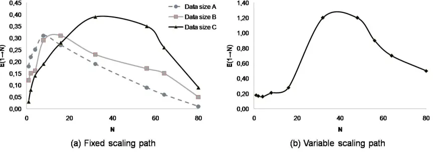
The elasticity analysis has been performed following the proposed steps. The reference case (the minimum config-uration) has been set at N = 1 (one provisioned virtual machine), while the maximum service size has been deter-mined to beNmax=80 (due to the available infrastructure in the LazarusCloud and to the provided instance type). Two scaling paths have been followed: a fixed scaling path (when the scaling is performed only increasing the number of provisioned instances) and a variable scaling path (when the scaling takes advantage of the elasticity enablers, tuning the service as best as possible for eachN value, in our case, mainly increasing the data size).
Figures 2 and 3 summarize the results obtained with our experiments. First of all, the defined elasticity metric can be validated. The proposed metric is able to dynamically capture the four considered elasticity components (scalabil-ity, accuracy, time and cost) increasing its value when the analysed service is capable to increase its size keeping a bal-ance between performbal-ance and cost and making this adap-tation accurate and fast. And decreasing its value when the balance between performance and cost, the accuracy or the speed of the adaptation have worse behaviour. There-fore, the defined metric is reliable. But it is also easy to measure, repeatable (this has been demonstrated repeating each experiment twenty times and obtaining always similar elasticity values) and consistent (it can be applied in differ-ent contexts having always the same meaning and allowing therefore to establish comparisons and to draw conclusions).
The performed analysis allows us to draw other interest-ing conclusions. Figure 2 illustrates the elasticity analysis of the MonteCarlo benchmark. In figure 2(a) the elasticity analysis with the fixed scaling path has been performed for the three available data sizes (remember that with a fixed scaling path only the value ofNin increased at every step of the procedure). This figure shows a better initial behaviour of elasticity with data size A because in this case we have a more manageable data size in only one virtual instance, obtaining better values forP (due to better response times) than with data sizes B and C. But it can be observed how as
N is increased a plateau is reached in the elasticity value for the three considered benchmarks, this plateau arrives later (for larger N values) for the larger data sizes, able to effi-ciently take advantage of the available resources to a higher degree. And this plateau can be sustained longer, being ob-served on higher elasticity values in the case of the data size C. It has to be considered that at this point of the elastic-ity curve the scalabilelastic-ity and accuracy terms are dominant for the elasticity figure. However, after this plateau the ser-vice elasticity decreases withN in the three analysed cases until values near 0 are reached, because the scalability and the g(∆) values constantly decrease at every stage of the analysis (summarizing, there is too little workload for too many resources, as service size is increased from here the HPC service experiences severe effects of inaccuracy). Even more, when configurations with a larger number of virtual machines are handled,h(R) shows a worse performance be-cause service reconfigurations are more difficult to manage. Figure 2(b) shows the elasticity analysis with the variable scaling path, using the data size as a elasticity enabler dur-ing the evaluation procedure. With the data size increase during the analysis (beginning in the data size A and final-izing with a size equivalent to 8X data size C), the service scalability and accuracy terms are able to be almost constant at every stage. As the reconfiguration times do not worsen significantly, the elasticity can be significantly improved if it is compared to the values obtained with the fixed scaling path. Yet it should be noted that fromN = 56 the value of
g(∆) begins to drop and the decrease of this term begins to have a great influence on the elasticity values. Above this value ofN,h(R) shows a worse performance too and some service requests begin to be rejected (worsening theλ val-ues and therefore, the service scalability), having all these factors a negative influence on the elasticity values.
Figure 3 shows a similar behaviour for the fluid physics simulation benchmark but being more difficult to obtain a sustained elasticity plateau and having it at lower elastic-ity values due to the limitations intrinsic to the considered HPC service: the evaluated application is tightly-coupled, therefore, synchronous and communication sensitive due to frequent inter-processor communications. The limitations imposed by the communications’ pattern affect the elastic-ity values, mainly throughψ(due to the measuredPvalues) andh(R) (because the service reconfigurations are more dif-ficult to carry out).
5.3
Discussion
Figure 2: Montecarlo simulation service elasticity analysis with the two considered scaling paths
Figure 3: Fluid physics simulation service elasticity analysis with the two considered scaling paths
First, no assumptions about the cloud infrastructure, about the provisioning and management mechanisms or about the application are needed to quantify a service elasticity with the proposed metric. Only the ability to measure and/or to determine few easy parameters that the user knows or that are available through the service’s API or SLA is re-quired. Second, the elasticity definition has been kept sim-ple to avoid measurement and analysis overheads. Perhaps more accurate elasticity models could be defined, but many users and providers may not adopt them to make real-time decisions (as it is currently happening with complex and weighted sets of scalability, accuracy, speed and cost met-rics).
Third, the four essential components of elasticity have been considered in a single metric. And fourth, all the aspects affecting a service elasticity can be captured in a proper way through the proposed metric, we are now work-ing in evaluatwork-ing the different importance of identified elas-ticity enablers:
• On the end user’s side:
1. Problem size: It is well known that the problem size affects scalability, therefore, this enabler may affect theψvalue.
2. Virtual and Application provisioning mechanisms: These mechanisms are essential on cloud architec-tures to deploy and to manage users’ applications meeting the required level of elasticity. This en-abler may affectP,C, ∆ andR.
• On the provider’s side:
1. Resources granularity: The instance types, con-tainers, machine images or server types offered by providers in their service catalogues have a great influence on elasticity. The most important aspect to consider is if these types are fixed (pre-defined by the the provider) or if cloud users have certain degree of personalization to lease exactly the resources they need. This enabler may affect ∆.
pro-visioning mechanisms in an infinite resources con-text, once new resources are provisioned for a user they need a time to be ready to use and actu-ally available to work. And the third is the Re-source Provisioning mechanism used to allocate virtual machines or instances to physical hosts in the provider data center. All these enablers may affectλandR.
3. Billing model: In this case, the most important issues are the billing quantum, slice or period and the latencies used to upgrade the billing basis for a user. This enabler may affectC.
6.
CONCLUSIONS AND FUTURE WORK
Elasticity is an essential property of cloud computing but there is a lack of standard and simple elasticity metrics and analysis procedures. This lack of a single general elastic-ity metric makes difficult to consider elasticelastic-ity as a service level objective in SLAs, to compare and to select cloud ser-vices or to optimize provisioning decisions and management mechanisms in terms of elasticity to mention only some ex-amples. This paper has introduced a new elasticity metric capable of considering its four main components and the most important aspects influencing elasticity in most cur-rent cloud services avoiding evaluating complex models and equations. Although a single metric could be a too extreme synthesis in complex environments such as those related to cloud computing, our experiments performed on a private HPC cloud providing two different kinds of services demon-strate the suitability of this metric in cloud contexts. The proposed metric allows cloud users and providers to easily quantify and understand services elasticity in order to make their decisions, and this was our main goal when defining the new metric. This along with the fact that the proposed metric allows flexibility and personalization through the use of thef QoS, QoSfunction and a deep analysis of the elas-ticity of a cloud service, not only its punctual quantification, increases the chance for the adoption of our approach.
Currently we are extending our experiments to larger, less controlled and more complex architectures (using public cloud services) in order to perform an exhaustive validation of the proposed metric and analysis procedure and to better understand the identified elasticity enablers and their real influence on elasticity.
7.
REFERENCES
[1] M. Becker, S. Lehrigy, and S. Becker. Systematically deriving quality metrics for cloud computing systems. InProceedings of the 5th ACM/SPEC International Conference on Performance Engineering, 2015. [2] M. Beltran. Automatic provisioning of multi-tier
applications in cloud computing environments.The Journal of Supercomputing, 71(6):2221–2250, 2015. [3] P. C. Brebner. Is your cloud elastic enough?:
Performance modelling the elasticity of infrastructure as a service (IaaS) cloud applications. InProceedings of the 3rd ACM/SPEC International Conference on Performance Engineering, pages 263–266, 2012. [4] R. N. Calheiros, R. Ranjan, and R. Buyya. Virtual
machine provisioning based on analytical performance and QoS in cloud computing environments. In
Proceedings of the 40th International Conference on Parallel Processing, pages 295–304, 2011.
[5] E. Folkerts, A. Alexandrov, K. Sachs, A. Iosup, V. Markl, and C. Tosun. Benchmarking in the cloud: What it should, can, and cannot be. InSelected Topics in Performance Evaluation and Benchmarking Lecture Notes in Computer Science, volume 7755, pages 173–188, 2013.
[6] G. Galante and L. C. E. de Bona. A survey on cloud computing elasticity. InProceedings of the IEEE/ACM 6th International Conference on Utility and Cloud Computing, pages 263–270, 2012.
[7] J. L. Gustafson. Reevaluating Amdahl’s law. Communications of the ACM, 31(5):532–533, 1988. [8] S. Herbst, N. Kounev and R. Reussner. Elasticity in
cloud computing: What it is, and what it is not. In Proceedings of the 10th International Conference on Autonomic Computing, pages 23–27, 2013.
[9] K. Hwang, X. Bai, Y. Shi, M. Li, W.-G. Chen, and Y. Wu. Cloud performance modeling and benchmark evaluation of elastic scaling strategies.IEEE
Transactions on Parallel and Distributed Systems, pages 1–1, 2015.
[10] S. Islam, K. Lee, A. Fekete, and A. Liu. How a consumer can measure elasticity for cloud platforms. InProceedings of the 3rd ACM/SPEC International Conference on Performance Engineering, pages 85–96, 2012.
[11] P. Jogalekar and M. Woodside. Evaluating the scalability of distributed systems.IEEE Transactions on Parallel and Distributed Systems, 11(6):589–603, 2000.
[12] V. Kumar and V. N. Rao. Parallel depth first search. Part II: Analysis.International Journal on Parallel Programming, 16(6):501–519, 1987.
[13] S. Lehrig, H. Eikerling, and S. Becker. Scalability, elasticity, and efficiency in cloud computing: A systematic literature review of definitions and metrics. InProceedings of the 11th International ACM
SIGSOFT Conference on Quality of Software Architectures, pages 83–92, 2015.
[14] Z. Li, L. OBrien, H. Zhang, and R. Cai. On a catalogue of metrics for evaluating commercial cloud services. InProceedings of the ACM/IEEE 13th International Conference on Grid Computing, pages 164–173, 2012.
[15] D. Nussbaum and A. Agarwal. Scalability of parallel machines.Communications of the ACM, 34(3):57–61, 1991.
[16] X. Sun, Y. Chen, and M. Wu. Scalability of
heterogeneous computing. InProceedings of the 34th International Conference on Parallel Processing, pages 557–564, 2005.
[17] J. Weinman. Time is money: The value of on-demand. Technical report, Hewlett-Packard, 2011.