Sky-canopy border length, exposure and thresholding influence accuracy of hemispherical photography for complex plant canopies

ORIGINAL ARTICLE

Sky-canopy border length, exposure

and thresholding influence accuracy

of hemispherical photography for complex

plant canopies

Guo‑Zhang M. Song

_{, Kuo‑Jung Chao}

_{, David Doley}

_{and David Yates}

Abstract

Background: Hemispherical photography (HP) is a popular method to estimate canopy structure and understorey light environment, which analyses photographs acquired with wide view‑angle lens (i.e. fisheye lens). To increase HP accuracy, the approaches of most previous studies were to increase the preciseness of exposure and thresholding of photographs, while ours quantified effects of canopy properties (gap fraction and length of sky‑canopy border (SCB)) and errors of exposure and thresholding on the accuracy of HP.

Results: Through analysing photographs of real and model canopies, it was showed that HP inaccuracy resulted from the mismatch between exposure and thresholding rather than exposure or thresholding errors alone. HP inac‑ curacy was a function of the SCB length and the extent of exposure and thresholding errors, but independent of gap fraction.

Discussion: In photographs, SCBs are recorded as grey pixels which greyness is in between that of sky and canopy pixels. When there are exposure and thresholding errors, grey pixels are those prone to be misclassified in image analysis. Longer (vegetation with taller canopies) and wider (lower image sharpness) SCBs in photographs can both result in a higher amount of grey pixels and ultimately higher HP inaccuracy for a given extent of exposure and threshold errors.

Conclusions: Using lenses with view angle narrower rather than that of fisheye lens can shorten the SCB length in photographs and in turn reduce HP estimation inaccuracy for canopy structure and understorey light environment. Since short SCBs and low levels of exposure and thresholding errors can both result in low HP inaccuracy, to identify the true performance of new exposure and thresholding methods for HP, photographs recording canopies with long SCBs and acquired with fisheye lenses should be used. Because HP inaccuracy in a function of the amount of grey pix‑ els resulting from SCBs, the amount of these pixels in photographs can be used as a universal parameter to quantify canopy properties influential to HP estimation and in turn make cross‑study comparisons feasible.

Keywords: Canopy openness, Digital number, Gap fraction, Leaf area index, Mixed sky‑canopy pixel

© The Author(s) 2018. This article is distributed under the terms of the Creative Commons Attribution 4.0 International License (http://creat iveco mmons .org/licen ses/by/4.0/), which permits unrestricted use, distribution, and reproduction in any medium, provided you give appropriate credit to the original author(s) and the source, provide a link to the Creative Commons license, and indicate if changes were made.

Open Access

*Correspondence: mikesong@nchu.edu.tw

1 _{Department of Soil and Water Conservation, National Chung Hsing} University, Taichung 40227, Taiwan

Background

Using hemispherical photography (HP) to estimate can-opy parameter (e.g. cancan-opy gap fraction and leaf area index (LAI)) relies on correct exposure and threshold-ing of canopy hemispherical photographs (CHPs) (Beck-schäfer et al. 2013; Jonckheere et al. 2005; Rich 1990). If CHPs are overexposed or analysed with threshold val-ues that are too low, canopy gap fraction will be over-estimated and LAI will be underover-estimated (Zhang et al. 2005). Conversely, the underexposure of CHPs or appli-cation of too-high threshold values will result in under-estimated gap fraction and overunder-estimated LAI. Achieving correct exposure and thresholding are widely-recognised challenges in HP (Beckschäfer et  al. 2013; Jonckheere et al. 2005; Rich 1990). Most previous studies attempted to improve HP accuracy by increasing the preciseness of exposure and thresholding (Rich 1990; Zhang et al. 2005). Identifying mechanisms of how exposure and threshold-ing errors influence HP accuracy can provide hints for novel approaches to raise HP accuracy.

There are multiple sources of grey pixels in CHPs. In CHPs, the desired sky and canopy pixels should appear white and black respectively. Nevertheless, some sky pix-els look grey because of thick cloud cover and low sky illumination created by the direction of sun radiation (Rich 1990). On the other hand, pixels recording bright leaves and light-coloured trunks appear grey. The other main source of grey pixels is the so-called mixed sky-can-opy pixels (hereafter mixed pixels) (Leblanc et al. 2005), which record portions of both sky and canopy in single pixels. Using regular grid cells to record digital images, widthless borders between two photographing objects (i.e. sky-canopy borders, SCBs, in the present study) are inevitably recorded as zones in which every single pixel contains images of these two objects (Fisher 1997). In the present study, these zones recording images of SCBs are defined as mixed-pixel zones (MPZs). Mixed pixels also include pixels recording images of linear (e.g. twigs) and small (e.g. small canopy openings) sub-pixel objects (Fisher 1997). Due to the nature of the grid pixel system of digital images, even with optically-perfect lens, the widthless SCBs are captured as MPZs which as wide as at least one pixel. Lens imperfections, image editing and operation errors (e.g. focusing failure, smudged lens, canopies moved by wind or camera shake) can blur SCBs and further increase the width of SCBs images.

Effects of exposure and thresholding errors on HP accuracy are exerted through their interactions with grey pixels in CHPs. Thresholding is a step of image analysis for HP, in which image pixels originally with a continu-ous greyness gradient are classified into either black or white pixels (binary images) by using a cut-off greyness (e.g. Rich 1990). Due to distinct differences between the

greyness of sky and canopy pixels, HP inaccuracy intro-duced by (manual or automatic) thresholding generally results from the misclassification of grey pixels rather than sky or canopy pixels. Therefore, the extent of HP inaccuracy resulting from thresholding errors should be a function of the grey-pixel fraction. Optimum exposure allows the image capture devices to capture the desired amount of light through manipulating shutter speed, lens aperture and light sensitivity (i.e. ISO value) of the device (Allen and Triantaphillidou 2011). In HP, blooming is an over-exposure effect in which excessive light causes light saturation on the sky pixels and pixels nearby, and in turn canopy gaps appear larger than they should be (Leblanc et  al. 2005). In other words, overexposure can result in that all grey pixels located between sky and canopy pixels (i.e. mixed pixels) appear as bright as sky pixels. Conse-quently, the extent of HP inaccuracy caused by exposure errors should also be a function of the grey-pixel fraction. Even though the misclassification of grey pixels has been widely recognised as a source of HP inaccuracy and vari-ous studies have developed new methods to classify them precisely (Hwang et al. 2016; Leblanc et al. 2005; Macfar-lane 2011; Macfarlane et al. 2014), few studies quantified their effects.

The effects of exposure and thresholding errors on HP estimation have to be examined together. The digi-tal number (also known as the greyness scale number) of all pixels in CHPs increases with exposure (Zhang et al. 2005). Nevertheless, as long as exposure is not high enough to cause the so-called blooming effect (Leblanc et  al. 2005), the effects of higher exposure on HP esti-mates can be cancelled out by using higher threshold val-ues in CHP analysis (Song et  al. 2014). In other words, an estimation inaccuracy cannot be introduced to HP by either exposure or thresholding errors alone, but by the mismatch between exposure and thresholding (hereafter, exposure-thresholding mismatch, ETM).

HP inaccuracy is likely a function of the ETM extent and two canopy properties (gap fraction and SCB length). Macfarlane et  al. (2000) and Macfarlane (2011) showed that, in Eucalyptus forests, the estimated LAI changed by 9–13% for each stop deviation from the correct exposure, suggesting that HP inaccuracy is a linear function of the ETM extent. Nevertheless, further studies are needed to show whether this relationship is applicable to other forest types. Macfarlane (2011) had reported a negative linear relationship between the grey-pixel fraction and canopy gap fraction. As mentioned above, pixels record-ing SCBs appear grey. Therefore, canopy gap fraction and SCB length may influence HP estimation through their effects on the grey-pixel fraction.

fraction, a model canopy system was used to minimise the sources of grey pixels and manipulate two canopy properties, SCB length and gap fraction, independently. Model canopies have been used in several HP studies because they are more controllable and manipulable than real canopies (Chianucci 2016; Hwang et al. 2016; Mac-farlane et al. 2014; Song et al. 2014). In the present study, model canopies were made with opaque black adhesive vinyl sheet, which diminished the amount of grey pixels caused by bright canopy elements; the greyness variation of sky pixels was controlled by using an artificial light source. The image size of smallest canopy elements and openings of model canopies were larger than the pixel size of the camera we used, which eliminated mixed pix-els resulting from sub-pixel objects. Consequently, in our model CHPs, the only source of grey pixels is mixed pix-els recording SCBs. This system also allowed us to vary SCB length and gap fraction independently, so that we could distinguish one’s effects from the other’s.

The present study aimed to improve HP accuracy through quantifying the relationships between canopy properties (SCB length and gap fraction), the grey-pixel fraction, the ETM extent and HP inaccuracy. We asked the following questions: (1) Is the grey-pixel fraction in a CHP a function of canopy gap fraction and SCB length? (2) Is the linear relationship between HP inaccuracy and the ETM extent (reported by Macfarlane (2011)) applica-ble to all forest types? (3) Can these two canopy proper-ties influence HP accuracy through their effects on the grey-pixel fraction?

Materials and methods

The grid model CHPs and real CHPs used in the present study were those in Song et al. (2014). For photographs showing the design of grid model canopies and image

acquisition devices of model CHPs, please refer to Song et al. (2014).

Design of model canopy

Model canopies were constructed from opaque black adhesive vinyl sheet (20 cm by 21 cm) with square open-ings of different dimensions, stuck to clear acrylic plastic to eliminate distortion during handling. A range of gap fraction and SCB length was simulated through varying the side length (L) of square openings and the separation width (W) of these openings (Fig. 1, Table 1). Gaps in real canopies were simulated by square openings, while black grids were the analogue of canopy elements (Fig. 1b). Designed gap fraction (GFd) is equal to L2/(L +W)2. For a desired combination of a given gap fraction and a side length of square opening, W can be acquired with the equation, W ₌₍L_/√GF_d)−L (Table 1).

Acquisition of CHPs

Three adapted CHP acquisition procedures were used to take photographs for the two-dimensional model

Fig. 1 Design of (a) the basic unit for (b) a model canopy (gap fraction = 0.5). L is the side length of square openings. W is the separation width between square openings

Table 1 Designed gap fraction (GFd) and  side length of square opening (L) of the 17 model canopies

The left and right values in each cell show the separation width between square openings (W; mm) and SCB length per unit area (B; mm mm−2_{) respectively.}

GFd = L2/(L + W)2. B = 4∙L/(L + W)2 Designed gap

fraction (GFd)

Side length of square opening (L) (mm)

2.50 5.00 10.00 20.00

0.05 8.68, 0.08 17.36, 0.04 34.72, 0.02 –, – 0.10 5.41, 0.16 10.81, 0.08 21.62, 0.04 –, – 0.25 2.50, 0.40 5.00, 0.20 10.00, 0.10 20.00, 0.05 0.50 1.04, 0.80 2.07, 0.40 4.14, 0.20 8.28, 0.10

canopies. First, model canopies backed with a piece of sand-scrubbed acrylic board (simulating the sky) was mounted at an end of a cylindrical pipe (internal diam-eter of 12.3 cm and length of 41 cm). The internal wall of this pipe was covered with black flannelette to reduce stray radiation. Second, a 28-watt ring fluorescent light (FLC-28, Falcon Eyes, Hong Kong, China) was placed behind the model sky to provide light for the model sky. A spot light meter (Spotmeter F, Konica Minolta, Tokyo, Japan) were used to make sure the illumination was even (illumination variation ≤ 0.2 stop) across the model sky and also measure the reference exposure from the model sky. Third, a Nikon D5000 camera (Tokyo, Japan) attached to Nikon AF-S ED 18–70 mm lens was mounted at the other end of the pipe. During the acquisition of model CHPs, the lens was always zoomed into 70 mm to reduce vignetting associated with wide view-angle lens. Through varying shutter speed but keeping aperture con-stant, CHPs for the 17 model canopies were taken with nine levels of exposure (− 3, − 2, − 1, 0, + 1, + 2, + 3, + 4 and + 5 stop) compensated from the reference exposure.

On 12 and 13 of August 2011, real CHPs were acquired in a forest about 500 m east of the Nanjenshan Research Station (22°05′05″N, 120°50′07″E) of Taiwan. Schefflera octophylla, Psychotria rubra, Castanopsis cuspidata var.

carlesii and Illicium arborescens were the most domi-nant tree species in this forest (Chao et al. 2010). CHPs were acquired with a 4.5  mm F2.8 circular fisheye lens (Sigma Corp., Kanagawa, Japan) mounted on the same Nikon D5000 camera which was used for the acquisi-tion of model CHPs. During the acquisiacquisi-tion of CHPs, the camera was mounted on a tripod to keep it 1  m above ground and reduce camera shake. To eliminate focus-ing failure associated with automatic focusfocus-ing, the focus of the fisheye lens was set to a constant distance, allow-ing that canopy elements more than 0.2  m away from the lens were included in the depth of field. Because CHPs acquired with the popular under-canopy exposure method (exposure of CHPs measured under canopy) tend to be overexposed (Chen et  al. 1991; Zhang et  al. 2005), we mainly examined the effects of overexposure on HP. Therefore, real CHPs were acquired with up to + 5 stop compensated from the reference exposure. Seven levels of exposure compensation were manipulated (− 1, 0, + 1, + 2, + 3, + 4 and + 5 stop) for every of the 46 pho-tographing locations and totally 322 CHPs were acquired. Before CHP acquisition for every location, the exposure for CHPs was measured with a Nikon D300 camera fol-lowing the above-canopy exposure method suggested by Zhang et al. (2005). This exposure-measuring camera was placed in an open area not farther than 0.5 km away from the CHP acquisition locations. This camera was attached

with a Nikon AF-S ED 18–70 mm lens and mounted on a tripod. The lens was pointed to the sky zenith and zoom out to 18 mm to cover most of the sky area. The desired aperture for exposure compensation of + 5 stop was obtained with the following settings: shutter-priority of camera mode, ISO 1600 of light sensitivity, 1/30 s of shut-ter speed and + 5 stop of exposure compensation. Using this aperture coupled with the same setting of light sensi-tivity and shutter speed on the CHP-acquisition camera could acquire CHPs with exposure compensations of + 5 stop. CHPs of exposure compensations of + 4, + 3, + 2, + 1, 0 and − 1 stop were acquired by keeping aperture constant but using shutter speeds of 1/60, 1/125, 1/250, 1/500, 1/1000 and 1/2000  s respectively. During CHP acquisition, all the following settings remained constant, including image format (Jpeg), image size (4288 × 2848 pixels), image quality (fine), metering mode (matrix), sensitivity to light (ISO 1600), colour mode and white balance (cloudy sky).

Quantifying the grey‑pixel fraction and SCB length

The method of Leblanc et  al. (2005) was modified to quantify the grey-pixel fraction in our CHPs. Sharp turns of curves in the greyness histograms of CHPs were used to visually identify the low threshold value separat-ing canopy and grey pixels and the high threshold value separating sky and grey pixels. Our method differed from that of Leblanc et al. (2005) in that the scale of the y axis (pixel fraction) of our histograms was linear rather than logarithmic. The grey-pixel fraction was the propor-tion of pixels with digit numbers between the low and high threshold values. Macfarlane (2011) has proposed an automatic method (two-corner method) using two humps of greyness histograms to identify the low and high threshold values. This method was not used in the present study because many greyness histograms of our CHPs had only one hump due to overexposure or low canopy gap fraction.

to the pixel grid to detect sharp greyness changes for two dimensional images (Ferreira and Rasband 2012). The MPZ length of a CHP is the proportion of pixels in MPZs (hereafter, pixel fraction of MPZ). Analyses showed that the MPZ length obtained through this method was a close approximation of SCB length per unit area (Addi-tional file 1: Figure S1).

Assessing HP inaccuracy associated with the ETM

Because exposure and thresholding of CHPs can have both independent and interacting effects on HP accuracy (Song et al. 2014), these two processes should be exam-ined together. A uniform basis for comparison of CHP exposure and thresholding effects was achieved by using two parameters, exposure manipulation and thresh-olding manipulation. Exposure manipulation was the extent of exposure deviating from the reference exposure measured under an unobscured overcast sky. Threshold-ing manipulation was transformed from the grey-scale threshold value using the regression model established by Song et al. (2014), in which the relationship between exposure manipulation (X) and the optimal threshold value (Y) is Y= 260.542/(1 + e(−X+1.422)/1.160_{). This model} determines the optimal threshold values for CHPs exposed with specific exposure manipulations. If a CHP is analysed with a threshold value which is the optimal threshold value for CHPs acquired with exposure manip-ulation of S stop, this CHP is analysed with thresholding manipulation of S stop. For example, the optimal thresh-old value for CHPs acquired with exposure manipulation of + 3 stop is 202. When a CHP is analysed with a thresh-old value of 202, its threshthresh-olding manipulation is + 3 stop. The ETM extent can be quantified by subtracting the thresholding manipulation from the exposure manip-ulation. When the ETM extent of a CHP is 0 stop, that means this CHP is analysed with its optimal threshold value and it can provide a correct estimate for HP. Posi-tive ETM extents indicate that CHPs are overexposed or analysed with threshold values that are too low, so that gap fraction is overestimated. Negative ETM extents underestimate gap fraction, as a result of underexposing CHPs or analysing CHPs with threshold values that are too high.

Because gap fraction is the HP estimation with the most direct connection between image and estimate (Jonckheere et al. 2005), we used gap fraction to evalu-ate the influence of grey pixels on HP inaccuracy. Prior to image analysis, the colour model and real CHPs were transformed into 8-bit greyscale images first. For model canopies, the correct gap fraction was obtained by ana-lysing scanned images of model canopies (GFs) (details in Additional file 1: Text S1). To obtain photographed gap fraction (GFp) estimated with different thresholding

manipulations, the amount of pixels for each digit num-ber was obtained for every model CHP with the function of “Histogram” of ImageJ version 1.43 (Abramoff et  al. 2004). Photographed gap fraction for the threshold value

i (GFpi) was obtained through dividing the total num-ber of pixels with digit numnum-bers ≥i by the total number of pixels in the circular images of CHPs. Using the rela-tionship between optimal threshold value and thresh-old manipulation, we could obtain gap fraction under different thresholding manipulations for every model CHP. The estimation inaccuracy of model CHPs (Im) was obtained by subtracting the correct gap fraction from the photographed gap fraction (Im=GFp −GFs).

For real canopies, the correct gap fraction was obtained by processing CHPs with matched exposure manipulation and thresholding manipulation (GFmatch). The estimation inaccuracy of real CHPs (Ir) was obtained by subtracting the correct gap fraction from the gap fraction obtained with a mismatch combination of exposure and threshold-ing manipulations (GFmismatch) (Ir=GFmismatch −GFmatch). This method for obtaining correct estimates can ensure that the ETM is the only source of estimation inaccuracy. If correct estimates are obtained with other often-used approaches (such as diffuse light transmittance obtained with quantum sensors), additional sources of estimation inaccuracy (e.g. differences between instruments) may obscure the relationship between HP inaccuracy and the ETM.

Data analysis

The F-test was used to evaluate the slope difference of regression lines with zero intercept, including regres-sion lines between the SCB length and HP inaccuracy, and between the MPZ length and HP inaccuracy. It is assumed that there are totally n observations in k groups. The total sum of square (SST) is the sum of square for residuals between observations and the grand regression line. The sum of square within groups (SSW) is the sum of square for residuals between observations in the same groups and the group-specific regression lines. The sum of square between groups (SSB) is obtained by subtract-ing SSW from SST (Sokal and Rohlf 1995). The degree of freedom within groups (DFW) and between groups (DFB) is equal to n −k and k − 1 respectively (Sokal and Rohlf 1995). F values are calculated where.

Data analyses and significance tests in the present study were conducted with Microsoft Excel 2010 (Redmond, Washington, US).

(1)

F_{value =} Mean square among groups Mean square within groups =

SSB/DFB

Results

The relationship between the grey-pixel fraction and canopy gap fraction was hump-shaped (Figs. 2 and 3). The coefficients of determination (r2_{) for fitting this} rela-tionship with linear models were lower than with hump-shaped models (Additional file 1: Figures S2 and S3). In contrast, the grey-pixel fraction was linearly related to the SCB length and MPZ length, but independent of can-opy gap fraction (Figs. 4 and 5).

Panels in the same columns of Fig. 6 show binary images which exposure manipulation is kept constant but thresholding manipulation is varied. Panels in the same rows of Fig. 6 shows binary images which thresholding manipulation is kept constant but exposure manipula-tion is varied. As long as the ETM extent is kept constant, even though the exposure manipulation and thresholding manipulation paired together vary, the amount and spa-tial distribution of misclassified pixels are almost identi-cal (e.g. Fig. 6e, j, o, t, m, r, w, ab). This indicates that the amount of misclassified pixels is not determined solely by either exposure manipulation or thresholding manipula-tion, but the ETM extent (Fig. 6). When the ETM extent is lower than − 1 stop, all pixels of model CHPs are

classified as canopy pixels (Fig. 6q, u, v, y, z, aa). When the ETM extent ranges from − 1 to + 3 stop, those mis-classified pixels were all located on where sky and canopy elements meet (Fig. 6e, i, j, m, n, o, r, s, t, w, x, ab). That is, misclassified pixels were those pixels recording SCBs. Once the ETM extent reached + 5 stop, a great propor-tion of canopy pixels (pixels of grids) are misclassified as sky pixels (Fig. 6f, k, p). All pixels are classified as sky pix-els, when the ETM extent is equal to or greater than + 7 stop (Fig. 6g, h, l).

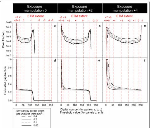
Panels a–c in Figs. 7 and 8 show greyness histograms (the frequency distribution of pixel fraction along the greyness gradient) of model and real CHPs respectively. In Figs. 7a–c, 8a–c, every curve has two humps. Humps at lower digital numbers are contributed by canopy pix-els, whereas humps at higher digital numbers are con-tributed by sky pixels. Pixels in between these two humps are the grey pixels. The grey pixel fraction increases with increasing SCB length (Fig. 7a–c) and MPZ length (Fig. 8a–c). Panels d–f in Figs. 7 and 8 show gap frac-tion estimated with threshold values from 0 to 255. As long as threshold values within the greyness range of grey pixels (ETM extent from − 1 to + 3 stop) are used

for thresholding (i.e. only grey pixels are misclassified), estimated gap fraction increases with ETM extents (Figs. 7d–f and 8d–f).

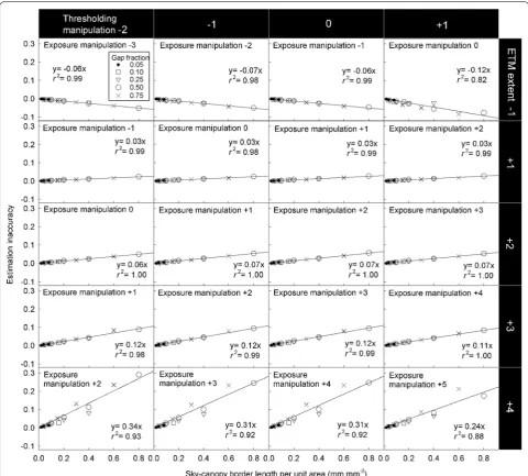
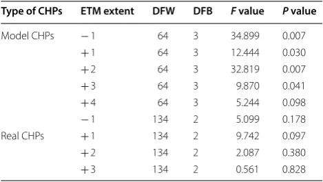
As long as only grey pixels are misclassified (i.e. the ETM extent is not zero and ranges from − 1 to + 3 stop), HP inaccuracy is positively related to the SCB length (Fig. 9) and MPZ length (Fig. 10). However, the HP inaccuracy is independent of canopy gap fraction for both model and real CHPs (Figs. 9 and 10). Signifi-cant tests showed that slopes of most regression lines with the same ETM extents (panels within the same rows in Figs. 9 and 10) differed significant in Fig. 9 (Table 2). This was a surprising result especially for regression lines within the same ETM extents of + 1 to + 3 stop in Fig. 9, because their slopes were almost identical. This result was attributed to that our control on the light intensity of the light source was not precise enough during the acquisition of model CHPs. For the detailed explanation, please see Additional file 1: Text S2. In panels within the same columns in Figs. 9 and 10, the slopes of regression lines approximately doubled with each stop increase in the ETM extent, indicating a positive linear relation-ship between HP inaccuracy and the ETM extent in both model and real CHPs.

Discussion

For ease of understanding, the mechanisms of how HP accuracy for canopy gap fraction is affected by canopy properties (gap fraction and SCB length), exposure and thresholding errors, and other factors are illustrated by a schematic diagram (Fig. 11).

Relationships between canopy properties, the grey‑pixel fraction, the ETM and HP inaccuracy

The relationship between canopy gap fraction and grey-pixel fraction is actually mediated by the SCB length (Fig. 11). Although the grey-pixel fraction was related with canopy gap fraction (Figs. 2 and 3), this relation-ship became negligible if the SCB length (Fig. 4) or MPZ length (Fig. 5) was included. Moreover, in the model canopy system, the SCB length and gap fraction could be varied independently (Table 1, Additional file 1: Figure S4). These results indicated that the relationship between gap fraction and the SCB length in Figs. 2 and 3 is a ten-dency rather than a cause-and-effect relationship, so is the relationship between gap fraction and the grey-pixel fraction (Fig. 11).

rather than linear (as reported by Macfarlane (2011)). When canopy gap fraction is zero or one, because of the absence of either sky or canopy elements, the SCB length has to be zero, and so do the MPZ length in CHPs. Con-sequently, if CHPs are sorted with gap fraction from zero to slightly higher values, the MPZ lengths of these CHPs increase from zero to greater values. If CHPs are sorted with gap fraction from one to slightly lower values, the MPZ lengths of CHPs also increase from zero to greater values. In summary, the relationship between canopy gap fraction and the grey-pixel fraction has to be hump-shaped. The study of Macfarlane (2011) was conducted in forests with relatively high canopy gap fraction (approxi-mately ranging from 0.15 to 0.6), he therefore observed the negative relationship near the higher end of the gap fraction gradient.

The mixed-pixel fraction is a function of not only the length but also the width of MPZs (Fig. 11). In images, the width of edges between two different objects (i.e. the MPZ width in the present study) decreases with the increase of image sharpness (Allen and Triantaphillidou 2011; Smith 1997) (Fig. 11). As mentioned in the intro-duction, even with optically-perfect lens, MPZs are at least as wide as one pixel due to the grid pixel system of digital images (Fisher 1997). Because image resolu-tion of the image capturing devices in many up-to-date

digital cameras exceeds that of lens (https ://www.dxoma rk.com/Revie ws/Looki ng-for-new-photo -gear-DxOMa rk-s-Perce ptual -Megap ixel-can-help-you, 20th April, 2017), blurred SCBs caused by lens imperfections are recorded in details, resulting in that MPZs are even wider. In addition, image sharpness is also influenced by the image-processing algorithms of camera firmware and operation errors during image acquisition (Allen and Tri-antaphillidou 2011) (Fig. 11). Effects of lens and firmware can be controlled by using the same hard- and soft-ware respectively. In contrast, effects of operations during image acquisition can vary greatly shot by shot. When taking CHPs, HP users should minimise the commonly-encountered operation errors, including focusing failure, smudged lens, canopy movement caused by wind and camera shake (Fig. 11).

In a CHP, the relationships among the overall grey-pixel fraction (F), the SCB length (B), image sharpness (S) and the fraction of grey pixels recording what else other than SCBs (G) can be summarised by Eq. 2. In practice, image sharpness of CHPs can be quantified with the 10–90% edge response distance, which is a parameter measuring the distance required for the edge response rising from 10 to 90% of the greyscale amplitude (Smith 1997).

(2)

F ₌B/S₊G

Even in real CHPs, grey pixels consist mainly of pixels recording SCBs. Due to the model canopy properties mentioned in the introduction, grey pixels record-ing what else other than SCBs (G) is eliminated from model CHPs, giving rise to almost perfectly linear rela-tionships between the overall grey-pixel fraction (F) and the SCB length (B) (Fig. 4, Eq. 2). Because bright canopy elements and dark skies are inevitable proper-ties of real CHPs (Rich 1990), G must be higher in real CHPs than in model CHPs. Consequently, coefficients of determination in Fig. 5 are lower than those in Fig. 4. In other words, high G weakens the linear relationship

between F and B (Eq. 2). Nevertheless, except exposure manipulation of + 5 stop, all coefficients of determina-tion in Fig. 5 were greater than 0.75, indicating that the majority of grey pixels in real CHPs are pixels record-ing SCBs. In other words, G in real CHPs is low enough so that the linear relationships between F and B are observed in Fig. 5. Exposure manipulation of + 5 stop raised the digit number of canopy elements to the level that many canopy pixels were recognised as grey pixels and in turn weakened the linear relationship between F

and B (Fig. 5).

Fig. 5 Relationships between the grey‑pixel fraction and the mixed‑pixel zone length in real CHPs. The pixel fraction of mixed‑pixel zone is an approximation of the SCB length. The unit of the exposure manipulation is stop

(See figure on next page.)

Fig. 6 Cropped binary images of model CHPs with the ETM extents ranging from − 7 to + 9 stop. (a)–(d) are the original images of model CHPs acquired with exposure manipulation of − 2, 0, + 2 and + 4 stop. (e)–(ab) are the binary images obtained with combinations of 4 exposure manipulations (− 2, 0, + 2, and + 4 stop) and 6 thresholding manipulations (− 5, − 3, − 1, + 1, + 3, and + 5 stop). Canopy and grey pixels which are misclassified as sky pixels are shown in red; sky and grey pixels which are misclassified as canopy pixels are blue; sky and grey pixels which are correctly classified as sky are white; canopy and grey pixels which are correctly classified as canopy are black. These CHPs were taken for a model canopy with gap fraction of 0.25 and SCB length per unit area of 0.4 mm mm−1 _{(i.e. side length of square opening of 2.5 mm). The diameter of}

As long as only grey pixels are misclassified, Eq. 3 bel-low can summarise the relationship between HP inac-curacy (I) and its influential factors (M, ETM extent;

F, the overall grey-pixel fraction; B, the SCB length; S, image sharpness; G, the fraction of grey pixels resulting from what else other than the SCBs) in Figs. 4, 5, 9 and 10.

The linear relationship between the ETM extent and HP inaccuracy is applicable for all forest types. In addi-tion to studies of Macfarlane et al. (2000) and Macfarlane

(3)

I ₌M_·F ₌M _·(B_/S₊G₎

and present studies indicated that this linear relationship is applicable to all forest types.

Suggestions for operations and future studies of HP The lack of precision on exposure and thresholding can lead to higher HP inaccuracy for images with long than short sky-canopy borders (Figs. 9 and 10). There is a need to know what kind of canopies are of long SCBs. Plants with taller canopies tend to have longer SCBs. When doubling the camera-to-canopy distance, the SCB length in captured images increases by a factor of two (Additional file 1: Figure S4), so do the grey-pixel

fraction. In other words, the taller the canopies (i.e. the greater camera-to-canopy distance), the higher the grey-pixel fraction of captured CHPs. Therefore, when exposure manipulation was controlled, HP inaccuracy increased with the distance between model canopies and the camera (Fig. 4 of Macfarlane et  al. (2014)). Trees with smaller leaf sizes and higher degrees of leaf division may have more openings and in turn longer SCBs in their canopies (Fig. 11). Further studies are needed to identify effects of leaf size and leaf division on the SCB length in acquired images.

The MPZ length has the potential to be a universal parameter, which enable researchers to quantify the effects of canopy properties which are influential to HP estimation and in turn carry out cross-study compari-sons for HP studies. Most HP researchers are aware that HP estimation is likely to be affected by species- and site-specific canopy properties, so they described where CHPs were taken and species composition and structure (e.g. stem density, tree height) of vegetation (e.g. Hwang et  al. 2016; Jonckheere et  al. 2005; Zhang et  al. 2005). Nevertheless, these attributes provide little insight into how and to what extent they may affect HP accuracy.

the SCB length can quantify effects of canopy proper-ties which can affect HP estimation. To facilitate cross-study comparisons, the MPZ length of CHPs should be provided in studies which use or develop the technique of HP.

The SCB length in photographs can be reduced through using lens with a narrower view angle. Although SCB length is an unmanipulable canopy property, SCB length captured by photographs can vary with lens’ view angle (Additional file 1: Figure S4). Cover photography developed by Macfarlane et al. (2007) uses lens with view angle narrower than that of the fisheye lens to acquire

photographs for LAI estimation. When taking photo-graphs for the same canopies, the narrower the lens’ view angle, the smaller fraction of canopies is captured, as a result, the shorter SCBs are recorded in photographs (Additional file 1: Figure S4). Because the grey-pixel frac-tion, a function of the SCB length (Fig. 4), of cover photo-graphs was lower than that of hemispherical photophoto-graphs (Chianucci 2016; Macfarlane 2011), estimation derived from cover photographs are more accurate than that based on hemispherical photographs (Chianucci 2016).

exposure and thresholding are the key to reduce negative effects of grey pixels on HP estimation. As mentioned in the introduction, it is infeasible to eliminate grey pix-els which record SCBs. However, HP inaccuracy caused by the misclassification of grey pixels can be mini-mised through reducing the ETM extent (Fig. 11; Eq. 3). Although extra efforts needed to establish the relation-ship between exposure and thresholding in advance, the exposure-corresponding method (Song et al. 2014) is one of the few objective methods which can integrate pro-cesses of exposure and thresholding and in turn reduce the ETM extent. Individually carrying out exposure and thresholding with correct methods is another approach to achieve accurate exposure and thresholding. Song et al. (2014) showed that using auto-thresholding meth-ods to analyse CHPs with exposure of one to two stop higher than the reference exposure measured from an unobscured overcast sky (the so-called above-canopy exposure method (Zhang et  al. 2005)) can also provide accurate HP estimation. Compared with the exposure-corresponding method, the advantage of this approach is that there is no need to establish the relationship between exposure and thresholding.

Manual thresholding is not recommended for studies which need high HP accuracy (e.g. monitoring temporal dynamics of understorey light environment in the same locations). Our results showed that the misclassified pix-els in binary images is hardly detectable even when the ETM extent is up to + 3 stop (Fig. 6e, j, o, t). For example, Fig. 6o shows the binary image which was acquired with

exposure manipulation of + 2 stop (its optimal threshold value is 162 (Song et al. 2014)) and analysed with thresh-olding manipulation of − 1 stop (that is, thresholding value of 28 was used (Song et al. 2014)). Even though the threshold value mismatch is as much as 134 (i.e. the ETM extent is + 3), the presence of misclassified grey pixels is barely noticeable if they are not coloured in red (Fig. 6o). On the other hand, the amount of grey pixels can account for as much as 10–15% of the total pixel number in real CHPs (Fig. 5) (Macfarlane 2011). This circumstance cou-pled with the misclassification of the majority of grey pixels will result in considerable HP inaccuracy. For example, when the ETM extent is + 3 stop, for half (23 out of 46) of our real CHPs source locations, the esti-mated gap fraction is more than twice the correct gap fraction (Additional file 1: Figure S5). In summary, it is very likely that estimates for gap fraction already deviate too much from correct ones before the grey-pixel mis-classification reaches to the visually-detectable extent. As mentioned previously, for studies which require high HP accuracy, auto-thresholding methods used with the above-canopy exposure method (Zhang et al. 2005) and the exposure-corresponding method (Song et  al. 2014) are recommended.

For studies developing exposure and thresholding methods for HP, photographs with long SCBs (i.e. pho-tograph which are acquired with wide view-angle lenses and record long SCB canopies) should be used. As men-tioned above, in terms of LAI estimation, cover photo-graphs outperform CHPs because the former contain fewer grey pixels recording SCBs (Chianucci 2016). Our results also showed that the shorter the SCBs, the lower the HP inaccuracy (Fig. 11; Eq. 3). In other words, low HP inaccuracy is the result of not only the good perfor-mance of exposure and thresholding methods, but also short SCBs in photographs used for performance evalu-ation. To ensure that the true performance of exposure and threshold methods is identified, their performance evaluation should be carried out with photographs with long SCBs rather than cover photographs.

Conclusions

The present study aims to identify how canopy proper-ties (gap fraction and SCB length) and errors of opera-tion (exposure and thresholding) influence an image property (grey-pixel fraction) of CHPs and ultimately affect HP estimation for gap fraction. Grey pixels in Table 2 Significant tests for  slopes of  regression models

with the same ETM extents

These regression model are shown in Figs. 9 and 10

CHP canopy hemispherical photograph, DFW degree of freedom within groups, DFB degree of freedom between groups

Type of CHPs ETM extent DFW DFB F value P value

Model CHPs − 1 64 3 34.899 0.007

+ 1 64 3 12.444 0.030

+ 2 64 3 32.819 0.007

+ 3 64 3 9.870 0.041

+ 4 64 3 5.244 0.098

− 1 134 2 5.099 0.178

Real CHPs + 1 134 2 9.742 0.097

+ 2 134 2 2.087 0.380

CHPs include pixels recording darkened sky, bright canopy elements, sub-pixel canopy elements and SCBs. Our results showed that exposure and threshold-ing errors cause the misclassification of grey pixels in binary images and in turn result in the HP inaccuracy. Moreover, the grey-pixel fraction of CHPs is a linear function of the SCB length because the majority of grey pixels are those recording SCBs. As a result, HP inac-curacy increases linearly with the SCB length of CHPs once there are exposure and thresholding errors. The relationship between canopy gap fraction and the grey-pixel fraction is, in fact, mediated by the SCB length. Results also showed that the linear relationship between

HP inaccuracy and the extent of exposure and thresh-olding errors is applicable to all forest types. Compared with hemispherical photographs, cover photographs which are acquired with narrow view-angle lenses can provide more accurate estimation for HP, because nar-row view-angle lenses capture only a small fraction of canopies and in turn shortens the SCB length in photo-graphs. Due to the fact that short SCBs in photographs and low levels of exposure and thresholding errors can both result in low HP inaccuracy, using photographs with long SCBs rather than cover photographs can ensure that the true performance of new exposure and thresholding methods for HP is identified.

Additional file

Additional file 1: Figure S1. Relationship between the sky‑canopy border length and mixed‑pixel zone length in model canopy hemispheri‑ cal photographs. Figure S2. Using linear models to fit the relationships between the grey pixel fraction and canopy gap fraction in model canopy hemispherical photographs. Figure S3. Using linear and second order polynomial models to fit the relationships between the grey pixel fraction and canopy gap fraction in model canopy hemispherical photographs. Figure S4. Relationships of canopy gap fraction, the camera‑to‑canopy distance and lens’ view angle to the sky‑canopy border length. Figure S5. Effects of the exposure‑thresholding mismatch extents (ETM extents) on estimated gap fraction. Text S1. The method for obtaining the correct gap fraction for model canopies. Text S2. The impreciseness of our control on the light intensity of the light source when taking photographs for model canopies.

Abbreviations

CHP: canopy hemispherical photograph; ETM: exposure‑thresholding mis‑ match; HP: hemispherical photography; MPZ: mixed‑pixel zone; LAI: leaf area index; SCB: sky‑canopy border.

Authors’ contributions

GZMS designed and conducted the experiments and wrote the manuscript. KJC, DD and DY reviewed the manuscript. All authors read and approved the final manuscript.

Author details

1 _{Department of Soil and Water Conservation, National Chung Hsing Univer‑} sity, Taichung 40227, Taiwan. 2 _{International Master Program of Agriculture,} National Chung Hsing University, Taichung 40227, Taiwan. 3 _{Centre for Mined} Land Rehabilitation, The University of Queensland, Brisbane, QLD 4072, Australia.

Acknowledgements

We thank Dr. Peter Chesson’s suggestions for regression models and statistics. Chien‑Hui Liao and Po‑Chuen Kung have been very helpful for acquiring CHPs in the field.

Competing interests

The authors declare that they have no competing interests.

Consent for publication

Authors agree to the terms of the Springer Open Copyright and License Agreement.

Ethics approval and consent to participate

Not applicable, the study involves no human participants.

Funding

The study was supported by the Ministry of Science and Technology of Taiwan (Grant Nos. NSC102‑2313‑B‑415‑001 and MOST104‑2311‑B‑415‑002).

Publisher’s Note

Springer Nature remains neutral with regard to jurisdictional claims in pub‑ lished maps and institutional affiliations.

Received: 14 March 2018 Accepted: 17 July 2018

References

Abramoff MD, Magalhães PJ, Ram SJ (2004) Image processing with ImageJ. Biophotonics Int 11:36–42

Allen E, Triantaphillidou S (2011) The manual of photography. Focal Press, Oxford

Beckschäfer P, Seidel D, Kleinn C, Xu J (2013) On the exposure of hemispherical photographs in forests. iForest 6:228–237. https ://doi.org/10.3832/ifor0 957‑006

Chao KJ et al (2010) Lowland rainforests in southern Taiwan and Lanyu, at the northern border of Paleotropics and under the influence of monsoon wind. Plant Ecol 210:1–17

Chen JM, Black TA, Adams RS (1991) Evaluation of hemispherical photography for determining plant‑area index and geometry of a forest stand. Agric For Meteorol 56:129–143. https ://doi.org/10.1016/0168‑1923(91)90108 ‑3

Chianucci F (2016) A note on estimating canopy cover from digital cover and hemispherical photography. Silva Fenn 50:1–10

Ferreira T, Rasband W (2012) ImageJ user guide—IJ 1.46

Fisher P (1997) The pixel: a snare and a delusion. Int J Remote Sens 18:679–685 Hwang Y, Ryu Y, Kimm H, Jiang C, Lang M, Macfarlane C, Sonnentag O (2016)

Correction for light scattering combined with sub‑pixel classification improves estimation of gap fraction from digital cover photography. Agric For Meteorol 222:32–44

Jonckheere I, Nackaerts K, Muys B, Coppin P (2005) Assessment of automatic gap fraction estimation of forests from digital hemispherical photog‑ raphy. Agric For Meteorol 132:96–114. https ://doi.org/10.1016/j.agrfo rmet.2005.06.003

Leblanc SG, Chen JM, Fernandes R, Deering DW, Conley A (2005) Methodology comparison for canopy structure parameters extraction from digital hem‑ ispherical photography in boreal forests. Agric For Meteorol 129:187–207.

https ://doi.org/10.1016/j.agrfo rmet.2004.09.006

Macfarlane C (2011) Classification method of mixed pixels does not affect canopy metrics from digital images of forest overstorey. Agric For Mete‑ orol 151:833–840. https ://doi.org/10.1016/j.agrfo rmet.2011.01.019

Macfarlane C, Coote M, White DA, Adams MA (2000) Photographic exposure affects indirect estimation of leaf area in plantations of Eucalyptus globu-lus Labill. Agric For Meteorol 100:155–168. https ://doi.org/10.1016/S0168 ‑1923(99)00139 ‑2

Macfarlane C, Grigg A, Evangelista C (2007) Estimating forest leaf area using cover and fullframe fisheye photography: thinking inside the circle. Agric For Meteorol 146:1–12

Macfarlane C, Ryu Y, Ogden GN, Sonnentag O (2014) Digital canopy photogra‑ phy: exposed and in the raw. Agric For Meteorol 197:244–253. https ://doi. org/10.1016/j.agrfo rmet.2014.05.014

Rich PM (1990) Characterizing plant canopies with hemispherical photo‑ graphs. Remote Sens Rev 5:13–29. https ://doi.org/10.1080/02757 25900 95321 19

Smith SW (1997) The scientist and engineer’s guide to digital signal process‑ ing. California Technical Publishing, San Diego

Sokal RR, Rohlf FJ (1995) Biometry, 3rd edn. W. H. Freeman and Company, New York

Song G‑ZM, Doley D, Yates D, Chao K‑J, Hsieh C‑F (2014) Improving accuracy of canopy hemispherical photography by a constant threshold value derived from an unobscured overcast sky. Can J For Res 44:17–27. https :// doi.org/10.1139/cjfr‑2013‑0082

Thimonier A, Sedivy I, Schleppi P (2010) Estimating leaf area index in different types of mature forest stands in Switzerland: a comparison of methods. Eur J For Res 129:543–562