Volume 2007, Article ID 42761,15pages doi:10.1155/2007/42761
Research Article
Video Coding Using 3D Dual-Tree Wavelet Transform
Beibei Wang,1Yao Wang,1Ivan Selesnick,1and Anthony Vetro2
1Electrical and Computer Engineering Department, Polytechnic University, Brooklyn, NY 11201, USA 2Mitsubishi Electric Research Laboratories, Cambridge, MA 02139, USA
Received 14 August 2006; Revised 14 December 2006; Accepted 5 January 2007
Recommended by B´eatrice Pesquet-Popescu
This work investigates the use of the 3D dual-tree discrete wavelet transform (DDWT) for video coding. The 3D DDWT is an attractive video representation because it isolates image patterns with different spatial orientations and motion directions and speeds in separate subbands. However, it is an overcomplete transform with 4 : 1 redundancy when only real parts are used. We apply the noise-shaping algorithm proposed by Kingsbury to reduce the number of coefficients. To code the remaining signifi-cant coefficients, we propose two video codecs. The first one applies separate 3D set partitioning in hierarchical trees (SPIHT) on each subset of the DDWT coefficients (each forming a standard isotropic tree). The second codec exploits the correlation between redundant subbands, and codes the subbands jointly. Both codecs do not require motion compensation and provide better perfor-mance than the 3D SPIHT codec using the standard DWT, both objectively and subjectively. Furthermore, both codecs provide full scalability in spatial, temporal, and quality dimensions. Besides the standard isotropic decomposition, we propose an anisotropic DDWT, which extends the superiority of the normal DDWT with more directional subbands without adding to the redundancy. This anisotropic structure requires significantly fewer coefficients to represent a video after noise shaping. Finally, we also explore the benefits of combining the 3D DDWT with the standard DWT to capture a wider set of orientations.
Copyright © 2007 Beibei Wang et al. This is an open access article distributed under the Creative Commons Attribution License, which permits unrestricted use, distribution, and reproduction in any medium, provided the original work is properly cited.
1. INTRODUCTION
Video coding based on 3D wavelet transforms has the poten-tial of providing a scalable representation of a video in spapoten-tial resolution, temporal resolution, and quality. For this reason, extensive research efforts have been undertaken to develop efficient wavelet-based scalable video codecs. Most of these studies employ the standard separable discrete wavelet trans-form. Because directly applying the wavelet transform in the time dimension does not lead to an efficient representation when the underlying video contains objects moving in diff er-ent directions, motion-compensated temporal filtering is de-ployed in state-of-the-art wavelet-based video coders [1–4]. Motion compensation can significantly improve the coding efficiency, but it also makes the encoder very complex. Fur-thermore, the residual signal resulting from block-based mo-tion compensamo-tion is very blocky and cannot be represented by a frame-based 2D DWT efficiently. Hence, the newest scal-able video coding standard [5] still uses block-based trans-forms for coding the residual.
An important recent development in wavelet-related re-search is the design and implementation of 2D multiscale transforms that represent edges more efficiently than does
the separable DWT. Kingsbury’s dual-tree complex wavelet transform (DT-CWT) [6] and Do’s contourlet transform [7] are examples. The DT-CWT is an overcomplete transform with limited redundancy (2m: 1 form-dimensional signals).
This transform has good directional selectivity and its sub-band responses are approximately shift invariant. The 2D DT-CWT has given superior results for image processing ap-plications compared to the DWT [6,8]. In [9], the authors developed a subpixel transform domain motion-estimation algorithm based on the 2D DT-CWT, and a maximum phase correlation technique. These techniques were incorporated in a video codec that has achieved a performance compara-ble to H.263 standard.
linear operations. So even though it is nonseparable and free of some of the limitations of separable transforms, it inherits the computational efficiency of separable transforms.
A core element common to all state-of-the art video coders is motion-compensated temporal prediction, which is the main contributor to the complexity and error sensitiv-ity of a video encoder. Because the subband coefficients as-sociated with the 3D DDWT directly capture moving edges in different directions, it may not be necessary to perform motion estimation explicitly. This is our primary motivation for exploring the use of the 3D DDWT for video coding.
The major challenge in applying the 3D complex DDWT for video coding is that it is an overcomplete transform with 8 : 1 redundancy. In our current study, we choose to retain only the real parts of the wavelet coefficients, which still leads to perfect reconstruction, while retaining the motion selectivity. This reduces the redundancy to 4 : 1 [10].
To reduce the number of coefficients necessary for repre-senting an image, Reeves and Kingsbury proposed an itera-tive projection-based noise-shaping (NS) scheme [8], which modifies previously chosen large coefficients to compensate for the loss of small coefficients. We have found that noise shaping applied to the 3D DDWT can yield a more compact set of coefficients than from the 3D DWT [12]. The fact that noise shaping can reduce the number of coefficients to below that required by the DWT (for the same video quality) is very encouraging.
To code the retained coefficients, we must specify both the locations and amplitudes (sign and magnitude) of the retained coefficients. 3D SPIHT is a well-known embedded video-coding algorithm [13], which applies the 3D DWT to a video directly, without motion compensation, and offers spa-tial, temporal, and PSNR-scalable bitstreams. The 3D DDWT coefficients can be organized into four trees, each with the same structure as the standard DWT. Our first DDWT-based video codec (referred as DDWT-SPIHT) applies 3D SPIHT to each DDWT tree. This codec gives better rate-distortion (R-D) performances than the 3D DWT.
With the standard nonredundant DWT, there is very lit-tle correlation among coefficients in different subbands, and DWT-based wavelet coders all code different subbands sep-arately. Because the DDWT is a redundant transform, we should exploit the correlation between DDWT subbands in order to achieve high coding efficiency. Through statistical analysis of the DDWT data, we found that there is strong correlation about locations of significant coefficients, but not about the magnitude and signs.
Based on the above findings, we developed another video codec referred to as DDWTVC. It codes the significant bits across subbands jointly by vector arithmetic coding, but codes the sign and magnitude information using context-based arithmetic coding within each subband. Compared to the 3D SPIHT coder on the standard DWT, the DDWTVC also offers better rate-distortion performance, and is supe-rior in terms of visual quality [14]. Compared to the first
proposed DDWT-SPIHT, DDWTVC has comparable and slightly better performance.
As with the standard separable DWT, the 3D DDWT applies an isotropic decomposition structure, that is, for each stage, the decomposition only continues in the low-frequency subband LLL, and for each subband the number of decomposition levels is the same for all spatial and tem-poral directions. However, not only the low-frequency sub-band LLL, but also subsub-bands LLH, HLL, LHL, and so forth, include important low-frequency information, and may ben-efit from further decomposition. Typically, more spatial de-composition stages produce noticeable gain for video pro-cessing. But additional temporal decomposition does not bring significant gains and incurs additional memory cost and processing delay.
If a transform allows decomposition only in one di-rection when a subband is further divided, it will gen-erate rectangular frequency tilings, and is thus called anisotropic [15,16]. Based on these observations, we pro-pose a new anisotropic DDWT, and examine its application to video coding. The experimental results show that the new anisotropic decomposition is more effective for video repre-sentation in terms of PSNR versus the number of retained coefficients.
Although the DDWT has wavelet bases in more spatial orientations than the DWT, it does not have bases in the hor-izontal and vertical directions. Recognizing this deficiency, we propose to combine the 3D DDWT and DWT, to capture directions represented by both the 3D DDWT and the DWT. Combining the 3D DWT and DDWT shows slight gains over using 3D DDWT alone.
To summarize the main contributions, the paper mainly focuses on video processing using a novel edge and motion selective wavelet transform, the 3D DDWT. In this paper, we demonstrate how to select the significant coefficients of the DDWT to represent video. Two iterative algorithms for co-efficient selection, noise shaping, and matching pursuit are examined and compared. We propose and validate the hy-pothesis that only a few bases of 3D DDWT have significant energy for an object feature. Based on these properties, two video codecs using the DDWT are proposed and tested on several standard video sequences. Finally, two extensions of the DDWT are proposed and examined for video represen-tation.
The paper is organized as follows.Section 2briefly in-troduces the 3D DDWT and its advantage. Section 3 de-scribes how to select significant coefficients for video coding. Section 4investigates the correlation between wavelet bases at the same spatial/temporal location for both the signifi-cance map and the actual coefficients.Section 5describes the two proposed video codecs based on the DDWT, and com-pares the coding performance to 3D SPIHT with the DWT. The scalability of the proposed video codec is discussed in
Section 6. Section 7 describes the new anisotropic wavelet
2. 3D DUAL-TREE WAVELET TRANSFORM
The design of the 3D dual-tree complex wavelet transform is described in [10]. At the core of the wavelet design is a Hilbert pair of bases,ψhandψg, satisfyingψg(t)=H(ψh(t)).
They can be constructed using a Daubechies-like algorithm for constructing Hilbert pairs of short orthonormal (and biorthogonal) wavelet bases. The complex 3D wavelet is de-fined asψ(x,y,z) =ψ(x)ψ(y)ψ(z), whereψ(x)= ψh(x) +
jψg(x). The real part ofψ(x,y,z) can be represented as
ψa=RealPart
ψ(x,y,z)
=ψ1(x,y,z)−ψ2(x,y,z)−ψ3(x,y,z)−ψ4(x,y,z), (1)
where
ψ1(x,y,z)=ψh(x)ψh(y)ψh(z), (2)
ψ2(x,y,z)=ψg(x)ψg(y)ψh(z),
ψ3(x,y,z)=ψg(x)ψh(y)ψg(z),
ψ4(x,y,z)=ψh(x)ψg(y)ψg(z).
(3)
Note that ψ1(x,y,z), ψ2(x,y,z), ψ3(x,y,z), ψ4(x,y,z) are four separable 3D wavelet bases, and each can produce one DWT tree containing 1 low subband and 7 high subbands. Becauseψa is a linear combination of these four separable
bases, the wavelet coefficients corresponding to ψa can be
obtained by linearly combining the four DWT trees, yield-ing one DDWT tree containyield-ing 1 low subband, and 7 high subbands.
To obtain the remaining DDWT subbands, we take in addition to the real part of ψ(x)ψ(y)ψ(z), the real part of ψ(x)ψ(y)ψ(z), ψ(x)ψ(y)ψ(z), ψ(x)ψ(y)ψ(z), where the overline represents complex conjugation. This gives the fol-lowing orthonormal combination matrix:
⎡ ⎢ ⎢ ⎢ ⎣
ψa(x,y,z)
ψb(x,y,z)
ψc(x,y,z)
ψd(x,y,z) ⎤ ⎥ ⎥ ⎥ ⎦=
1 2
⎡ ⎢ ⎢ ⎢ ⎣
1 −1 −1 −1 1 −1 1 1 1 1 −1 1
1 1 1 −1
⎤ ⎥ ⎥ ⎥ ⎦ ⎡ ⎢ ⎢ ⎢ ⎣
ψ1(x,y,z) ψ2(x,y,z) ψ3(x,y,z) ψ4(x,y,z)
⎤ ⎥ ⎥ ⎥ ⎦. (4)
By applying this combination matrix to the four DWT trees, we obtain four DDWT trees, containing a total of 4 low subbands and 28 high subbands. Each high subband has a unique spatial orientation and motion.
Figure 1shows the isosurfaces of a selected wavelet from both the DWTFigure 1(a)and the DDWTFigure 1(b). Like a contour plot, the points on the surfaces are points where the function is equal valued. As illustrated inFigure 1, the wavelet associated with the separable 3D transform has the checkerboard phenomenon, a consequence of mixing of orientations. The wavelet associated with the dual-tree 3D transform is free of this effect.
Figure 2shows all the wavelets in a particular temporal frame for both the DWT and DDWT. In Figure 2(b), the wavelets in each row correspond to 7 high subbands con-tained in one DDWT tree. For 3D DDWT, each subband
(a) (b)
Figure1: Isosurfaces of a typical 3D DWT basis (a) and a typical 3D DDWT basis (b).
(a) 3D DWT
(b) 3D DDWT
Figure2: Typical wavelets associated with (a) the 3D DWT and (b) 3D DDWT in the spatial domain.
corresponds an image pattern with a certain spatial orien-tation and motion direction and speed. The motion direc-tion of each wavelet is orthogonal to the spacial orientadirec-tion. Note that the wavelets with the same spatial orientation in Figure 2(b)have different motion directions and/or speeds. For example, the second and third wavelets in the top row move in opposite directions. As can be seen, the 3D DWT can represent the horizontal and vertical features well, but it mixes two diagonal directions in a checkerboard pattern. The 3D DDWT is free of the checkerboard effect, but it does not represent the vertical and horizontal orientations in pursuit of other directions. The 3D DDWT has many more subbands than the 3D DWT (28 high subbands instead of 7, 4 low sub-bands instead of 1). The 28 high subsub-bands isolate 2D edges with different orientations that are moving in different direc-tions.
computational load of a block-based hybrid video coder and wavelet-based coders using separable DWT. If a video sequence contains differently oriented edges moving in dif-ferent directions and speeds, coefficients for the wavelets with the corresponding spatial orientation and motion pat-terns will be large. By applying the 3D DDWT to a video sequence directly, and coding large wavelet coefficients, we are essentially representing the underlying video as basic im-age patterns (varying in spatial orientation and frequency) moving in different ways. Such a representation is naturally more efficient than using a separable wavelet transform di-rectly, with which a moving object in arbitrary directions that are not characterized by any specific orientation and/or motion will likely contribute many small coefficients associ-ated with wavelets. Directly applying the 3D DDWT to the video is also more computationally efficient than first per-forming motion estimation and then applying a separable wavelet transform along the motion trajectory, and finally applying a 2D wavelet transform to the prediction error im-age. Finally, because no motion information is coded sepa-rately, the resulting bitstream can be fully scalable.
For the simulation results presented in the paper, 3-level wavelet decompositions are applied for both the 3D DDWT and 3D DWT. The 3D DWT uses the Daubechies (9, 7)-tap filters. For the DDWT, the Daubechies (9, 7)-tap filters are used at the first level, and Qshift filters in [6] are used beyond level 1.
3. ITERATIVE SELECTION OF COEFFICIENTS
For video coding, the 4 : 1 redundancy of the 3D DDWT (real parts) [10] is a major challenge. However, an overcom-plete transform is not necessarily ineffective for coding be-cause a redundant set provides flexibility in choosing which basis functions to use in representing a signal. Even though the transform itself is redundant, the number of the critical coefficients that must be retained to represent a video sig-nal accurately can be substantially smaller than that obtained with standard non-redundant separable transform.
The selection of significant coefficients from nonorthog-onal transforms, like DDWT, is very different from the or-thogonal transforms, like DWT. Because the bases are not orthogonal, one should not simply keep all the coefficients that are above a certain threshold and delete those that are less than the threshold. In this section, we compare the effi -ciency of two coefficient selection schemes, matching pursuit and noise shaping.
3.1. Matching-pursuit algorithm
Matching pursuit (MP) is a greedy algorithm to decompose any signal into a linear expansion of waveforms that are se-lected from a redundant dictionary of functions [17, 18]. These waveforms are selected to best match the signal struc-tures. The matching-pursuit (MP) algorithm is well known for video coding with overcomplete representations [19].
With the matching-pursuit (MP) algorithm, the signif-icant coefficients are chosen iteratively. Starting with all the
Video
DDWTy0 y i
θi
yi
Thresholding IDDWT xi +
− −
ei
k
DDWT
wi
+ Delay
yi+1=yi+wi
Figure3: Noise-shaping algorithm.
original coefficients for a given signal, the one with the largest magnitude is chosen. The error between the original sig-nal and the one reconstructed using the chosen coefficient is then transformed (without using the previously chosen basis function). The largest coefficient is then chosen from the resulting coefficients, and a new error image is formed and transformed again. This process repeats until the desired number of coefficients is chosen.
Because only one coefficient is chosen in each itera-tion, the computation is very slow. Our simulations (see Section 3.3) show that the matching pursuit only has slight gain over using theNlargest original DDWT coefficients di-rectly.
3.2. Noise-shaping algorithm
For nonorthogonal transforms like the DDWT, deleting in-significant coefficients can be modelled as adding noise to the other coefficients. In [20], the effect of additive noise in over-sampled filter bank systems is examined. Much of the alge-bra for the overcomplete DDWT transform analysis is similar with the polyphase domain analysis in [20]. Recognizing this, Reeves and Kingsbury proposed an iterative projection-based noise shaping (NS) scheme [8]. As illustrated inFigure 3, the coefficients are obtained by running the iterative projection algorithm with a preset initial threshold, and gradually re-ducing it until the number of remaining coefficients reaches N, a target number. In each iteration, the error coefficients are multiplied by a positive real number kand added back to the previously chosen large coefficients, to compensate for the loss of small coefficients due to thresholding.
NS requires substantially fewer computations than MP, to yield the set of coefficients that can yield the same represen-tation accuracy. This is because with NS, many coefficients can be chosen in one iteration (those that are larger than a threshold), whereas with MP, only one coefficient is chosen in each iteration.
24 26 28 30 32 34 36 38
PSNR
(dB)
2 2.5 3 3.5 4 4.5 5 5.5 6 6.5 7
×104
Number of nonzero coefficients DDWT NS
DDWT MP DDWT w/o NS
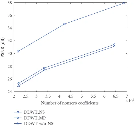
Figure 4: PSNR (dB) versus number of nonzero coefficients for the DDWT using noise shaping (DDWT NS, top curve), using matching pursuit (DDWT MP, middle curve), without noise shap-ing (DDWT w/o NS, lower curve) for a small size test sequence.
3.3. Simulation results
For a given number of coefficients to retain, N, the re-sults designated below as DWT and DDWT w/o NS are ob-tained by simply choosing theNlargest ones from the orig-inal coefficients. DDWT MP is obtained by selecting coef-ficients with MP. With DDWT NS, the coefficients are ob-tained by running the iterative projection noise-shaping al-gorithm with a preset initial threshold 256.0, and gradu-ally reducing it until the number of remaining coefficients reachesN. The reducing step is set as 1. The energy com-pensation parameter k is set as 1.8, which gives the best performance for all tested video sequences experimentally.
Figure 4 compares the reconstruction quality (in terms of
PSNR) using the same number of retained coefficients (orig-inal values without quantization) using different methods. Because the MP algorithm takes tremendous computation to deduce a large set of coefficients, this comparison is done using a small size (80×80×80 pixels) video sequence. The DDWT MP provides only marginal gain over simply choos-ing the largestNcoefficients (DDWT w/o NS). On the other hand, DDWT NS yielded much better image quality (5-6 dB higher) than DDWT w/o NS with the same number of coef-ficients.
Figure 5compares the reconstruction quality (in terms
of PSNR) using the same number of retained coefficients us-ing different methods (except for DDWT MP) for two stan-dard test sequences. The testing sequence “Foreman” is QCIF and “Mobile Calendar” is CIF. Both sequences have the same frame rate 30 fps and 80 frames are used for simulations.
Figure 5shows that although the raw number of coefficients
with 3D DDWT is 4 times more than DWT, this number
28 30 32 34 36 38 40
PSNR
(dB)
0.5 1 1.5 2 2.5 3
×105
Number of nonzero coefficients DDWT NS
DWT DDWT w/o NS
(a) Foreman (QCIF)
20 25 30 35 40 45
PSNR
(dB)
0 0.5 1 1.5 2 2.5 3
×106
Number of nonzero coefficients DDWT NS
DWT DDWT w/o NS
(b) Mobile Calendar (CIF)
Figure 5: PSNR (dB) versus number of nonzero coefficients for the DDWT using noise shaping (DDWT NS, upper curve), the DWT (middle curve), and the DDWT without noise shaping (DDWT w/o NS, lower curve).
Figure 5 shows that with DDWT NS, we can use fewer coefficients to reach a desired reconstruction quality than DWT. However, this does not necessarily mean that DDWT NS will require fewer bits for video coding. This is because we need to specify both the location as well as the value of each retained coefficient. Because DDWT has 4 times more coefficients, specifying the location of a DDWT coeffi -cient requires more bits than specifying that of a DWT co-efficient. The success of a wavelet-based coder critically de-pends on whether the location information can be coded ef-ficiently. As shown inSection 4.1, there are strong correla-tions among the locacorrela-tions of significant coefficients in dif-ferent subbands. The DDWTVC codec to be presented in Section 5.2exploits this correlation in coding the location in-formation.
4. THE CORRELATION BETWEEN SUBBANDS
Because the DDWT is a redundant transform, the subbands produced by it are expected to have nonnegligible correla-tions. Since wavelet coders code the location and magnitude information separately, we examine the correlation in the lo-cation and magnitude separately.
4.1. Correlation in significant maps
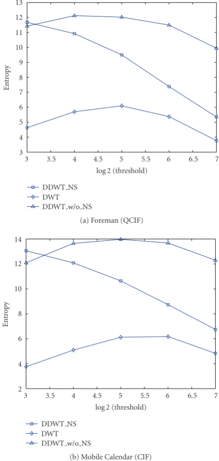
We hypothesize that although the 3D DDWT has many more subbands, only a few subbands have significant energy for an object feature. Specifically, an oriented edge moving with a particular velocity is likely to generate significant coefficients only in the subbands with the same or adjacent spatial ori-entation and motion pattern. On the other hand, with the 3D DWT, a moving object in arbitrary directions that are not characterized by any specific wavelet basis will likely con-tribute to many small coefficients in all subbands. To validate this hypothesis, we compute the entropy of the vector con-sisting of the significance bits at the same spatial/temporal location across 28 high subbands. The significance bit in a particular subband is either 0 or 1 depending on whether the corresponding coefficient is below or above a chosen thresh-old. The entropy of the significance vector will be close to 28 if there is not much correlation between the 28 subbands. On the other hand, if the pattern that describes which bases are simultaneously significant is highly predictable, the entropy should be much lower than 28. Similarly, we calculate the en-tropy of the significance bits across the 7 high subbands of DWT, and compare it to the maximum value of 7.
Figure 6 compares the vector entropy for significant
maps among the DWT, DDWT NS, and DDWT w/o NS, for varying thresholds from 128 to 8. The results shown here are for the top scale only—other scales follow the same trend. We see that, with DDWT, even without noise shap-ing, the vector entropy is much lower than 28. Moreover, noise shaping helps reduce the entropy further. In contrast, with DWT, the vector entropy is close to 7 at some thresh-old values. This study validates our hypothesis that the sig-nificance maps across the 28 subbands of DDWT are highly correlated.
3 4 5 6 7 8 9 10 11 12 13
Ent
ro
p
y
3 3.5 4 4.5 5 5.5 6 6.5 7 log 2 (threshold)
DDWT NS DWT DDWT w/o NS
(a) Foreman (QCIF)
2 4 6 8 10 12 14
Ent
rop
y
3 3.5 4 4.5 5 5.5 6 6.5 7 log 2 (threshold)
DDWT NS DWT DDWT w/o NS
(b) Mobile Calendar (CIF)
Figure 6: The vector entropy of significant maps using the 3D DWT, the DDWT NS, and the DDWT w/o NS, for the top scale.
4.2. Correlation in coefficient values
25 20 15 10 5
5 10 15 20 25 25 20 15 10 5
5 10 15 20 25 (a) Foreman (QCIF)
25 20 15 10 5
5 10 15 20 25 25 20 15 10 5
5 10 15 20 25 (b) Mobile Calendar (CIF)
Figure 7: The correlation matrices of the 28 subbands of 3D DDWT w/o NS (left) and DDWT NS (right). The grayscale is log-arithmically related to the absolute value of the correlation. The brighter colors represent higher correlation.
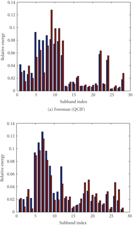
From these correlation matrices, we find that only a few sub-bands have strong correlation, and most other subsub-bands are almost independent. After noise shaping, the correlation be-tween subbands is reduced significantly. A greater number of subbands are almost independent from each other. It is inter-esting to note that, for the “Foreman” sequence (which has predominantly vertical edges and horizontal motion), bands 9–12 (the four subbands in the third column ofFigure 2) are highly correlated before and after noise shaping. These four bands have edges close to vertical orientations but all moving in the horizontal direction. For “Mobile Calendar,” these four bands also have relatively stronger correlations before noise shaping, but this correlation is reduced after noise shaping. Figure 8illustrates the energy distribution among the 28 sub-bands for the top scale with and without noise shaping. The energy distribution pattern depends on the edge and motion patterns in the underlying sequence. For example, the en-ergy is more evenly distributed between different subbands with “Mobile Calendar.” Further more, noise shaping helps to concentrate the energy into fewer subbands.
5. DDWT-BASED VIDEO CODING
In this section, we present two codecs: DDWT-SPIHT and DDWTVC. Both codecs do not perform motion estimation. Rather, the 3D DDWT is first applied to the original video di-rectly and the noise-shaping method is then used to deduce the significant coefficients. The two codecs differ in their
0 0.02 0.04 0.06 0.08 0.1 0.12 0.14
R
elat
iv
e
energ
y
0 5 10 15 20 25 30
Subband index (a) Foreman (QCIF)
0 0.02 0.04 0.06 0.08 0.1 0.12 0.14
R
elat
iv
e
energ
y
0 5 10 15 20 25 30
Subband index (b) Mobile Calendar (CIF)
Figure8: The relative energy of 3D DDWT 28 subbands with (the right column in each subband) and without noise shaping (the left column).
ways to code the retained DDWT coefficients. The DDWT-SPIHT codec directly applies the well-known 3D DDWT-SPIHT codec on each of the four DDWT trees. Hence it does not exploit the correlation crosssubbands in different trees. The second codec, DDWTVC, exploits the intersubband correla-tion in the significance maps, but code the sign and magni-tude information within each subband separately.
5.1. DDWT-SPIHT codec
have significant descendants with high probability (parent-children probability). To examine such correlation across dif-ferent scales in 3D DDWT, we evaluated the parent-children probability shown inFigure 9. We can see that there is strong correlation across scales with 3D DDWT, but compared to 3D DWT, the correlation is weeker. After noise shaping, this correlation is further reduced.
Based on the similar structure and properties with DWT, our first DDWT-based video codec applies 3D SPIHT [13] to each DDWT tree after noise shaping. As will be seen in the simulation results presented in Section 5.3, this simple method, not optimized for DDWT statistics, already outper-forms the 3D SPIHT codec based on the DWT. This shows that DDWT has the potential to significantly outperform DWT for video coding.
5.2. DDWTVC codec
In DDWTVC, the noise-shaping method is applied to deter-mine the 3D DDWT coefficients to be retained, and then a bitplane coder is applied to code the retained coefficients. The low subbands and high subbands are coded separately, each with three parts: significance-map coding, sign coding, and magnitude refinement.
5.2.1. Coding of significance map
As has been shown inSection 4.1, there are significant cor-relations between the significance maps across 28 high sub-bands, and the entropy of the significance vector is much smaller than 28. This low entropy prompted us to apply adaptive arithmetic coding for the significance vector. To uti-lize the different statistics of the high subbands in each bit-plane, individual adaptive arithmetic codec is applied for each bitplane separately. Though the vector dimension is 28, for each bitplane, only a few patterns appear with high prob-abilities. So only patterns appearing with sufficiently high probabilities (determined based on training sequences) are coded using vector arithmetic coding. Other patterns are coded with an escape code followed by the actual binary pat-tern.
For the four low subbands, vector coding is used to ex-ploit the correlation among the spatial neighbors (2×2 re-gions) and four low subbands. The vector dimension in the first bitplane is 16. If a coefficient is already significant in a previous bitplane, the corresponding component of the vec-tor is deleted in the current bitplane. After the first several bitplanes, the largest dimension is reduced to below 10. As with the high subbands, only symbols occurring with a suf-ficiently high probability are coded using arithmetic cod-ing. Different bitplanes are coded using separate arithmetic coders and different vector sizes.
The proposed video coder codes 3D DDWT coefficients in each scale separately. As illustrated inFigure 9, 3D DDWT does not have strict parent-children relationship as does the 3D DWT [13]. Noise shaping destroys such a relationship further. So the spatial-temporal orientation trees used in 3D SPIHT [13] are only applied in the finest stage, which has a lot of zero coefficients.
5.2.2. Coding of sign information
This part is used to code the sign of the significant coeffi -cients. Our experiments show that four low subbands have very predicable signs. This predictability is due to the par-ticular way the 3D DDWT coefficients are generated. Re-call the orthonormal combination matrix for producing the 3D DDWT given in (2). Because the original DWT low-subbands are always positive (because they are lowpass fil-tered values of the original image pixels) and the coefficients in different low subbands have similar values at the same lo-cation, based on the combination matrix, the low subband in the first DDWT tree is almost always negative, and the other three low subbands in the other three DDWT trees are almost all positive. We predict the signs of significant coefficients in low subbands according to the above observation, and code the prediction errors using arithmetic coding.
For high subbands, we have found that the current co-efficient tends to have the same sign as its neighbor in the lowpass direction, but have the opposite sign to its highpass neighbor. (In a subband which is horizontally lowpass and vertically high-pass, the lowpass neighbors are those to the left and right, and highpass neighbors are those above and below.) The prediction from the lowpass neighbor is more accurate than that from the highpass neighbor. The coded binary valued symbol is the product of the predicted and real sign bit. To exploit the statistical dependencies among adja-cent coefficients in the same subband, we apply the similar sign context models of 3D embedded wavelet video (EWV) [21].
5.2.3. Magnitude refinement
This part is used to code the magnitudes (0 or 1) of sig-nificant coefficients in the current bitplane. Because only a few subbands have strong correlation as demonstrated in
Section 4.2, the magnitude refinement is done in each
sub-band individually. The context modelling is used to explore the dependence among the neighboring coefficients. Context models similar to the EWV method [21] are applied to 3D DDWT here.
5.3. Experimental results of DDWT video coding
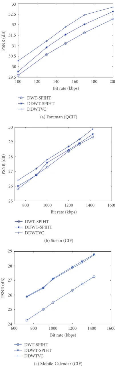
In this section, we evaluate the coding performance of the two proposed codecs, DDWT-SPIHT and DDWTVC. The comparisons are made to 3D SPIHT [13] using DWT (to be referred as DWT-SPIHT). None of these codecs use motion compensation. Only the comparisons of luminance compo-nentY are presented here. Two CIF sequences “Stefan” and “Mobile Calendar” and a QCIF sequence “Foreman” are used for testing. All sequences have 80 frames with a frame rate of 30 fps. Figure 10compares the RD performances of DWT-SPIHT and the two proposed video codecs, DDWTVC and DDWT-SPIHT.
Figure 10 illustrates that both DDWT-SPIHT and
0.1 0.2 0.3 0.4 0.5 0.6 0.7 0.8 0.9 1
P
robabilit
y
3 4 5 6 7 8 9 10 11 12
log 2 (threshold) DDWT NS
DWT DDWT w/o NS
Figure9: Probability that an insignificant parent does not have sig-nificant descendants for “Forman.”
video sequence which has many edges and motions, like “Mobile Calendar,” DDWTVC outperforms DWT-SPIHT more than 1.5 dB. DDW-TVC improves up to 0.8 dB for the “Foreman” and 0.5 dB better PSNR for “Stefan.” Consider-ing that DDWT has four times raw data than 3D DWT, these results are very promising.
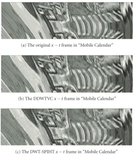
Subjectively, both DDWTVC and DDWT-SPIHT have better quality than DWT-SPIHT for all tested sequences. Coded frames by DDWTVC and DWT-SPIHT for a frame from the “Stefan” sequence are shown inFigure 11. We can see that DDWTVC preserves edge and motion informa-tion better than DWT-SPIHT; DWT-SPIHT exhibits blurs in some regions and when there are a lot of motions. The visual differences here are consistent with those in other sequences. When displayed as a video at real time (30 fps), the DWT-SPIHT coded video was found to exhibit annoying flicker-ing artifacts. To investigate the reason behind this, we show thex−tframes of decoded video, where anx−tframe is a horizontal cut of the video through time (as illustrated in Figure 12).Figure 13(a) illustrates the originalx−tframe, and (b) is the decoded x −t frame from DDWTVC, and (c) is the DWT-SPIHTx−tframe.Figure 13illustrates that the motion trajectory in the original and DDWTVC decoded x−tframes is much more smoother, but the DWT-SPIHT x−tframe has more zigzag characteristics, which might be the reason why the DWT-SPIHT coded video has flickering artifacts.
Recall that the DDWT-SPIHT codec exploits the spa-tial and temporal correlation within each subband while coding significance, sign, and magnitude information. The DDWTVC codec also exploits within subband correlation when coding the sign and magnitude information. But for the significance information, it exploits the intersubband correlation, at the expense of the intrasubband correlation.
29.5 30 30.5 31 31.5 32 32.5 33
PSNR
(dB)
100 120 140 160 180 200
Bit rate (kbps) DWT-SPIHT
DDWT-SPIHT DDWTVC
(a) Foreman (QCIF)
25 26 27 28 29 30
PSNR
(dB)
800 1000 1200 1400 1600
Bit rate (kbps) DWT-SPIHT
DDWT-SPIHT DDWTVC
(b) Stefan (CIF)
24 25 26 27 28 29
PSNR
(dB)
600 800 1000 1200 1400 1600
Bit rate (kbps) DWT-SPIHT
DDWT-SPIHT DDWTVC
(c) Mobile-Calendar (CIF)
(a) The 16th frame in “Stefan” reconstructed from DDWTVC
(b) The 16th frame in “Stefan” reconstructed from DWT-SPIHT
Figure11: The subjective performance comparison of DDWTVC and DWT-SPIHT for “Stefan.”
Our simulation results suggest that the exploiting interband correlation is equally, if not more, important as exploiting the intraband correlation. The benefit from exploiting the interband correlation is sequence dependent. A codec that can exploit both interband and intraband correlations is ex-pected to yield further improvement. This is a topic of our future research.
6. SCALABILITY OF DDWTVC
Scalable coding refers to the generation of a scalable (or em-bedded) bit stream, which can be truncated at any point to yield a lower-quality representation of the signal. Such rate scalability is especially desirable for video streaming applica-tions, in which many clients may access the server through access links with vastly different bandwidths.
The main challenge in designing scalable coders is how to achieve scalability without sacrificing the coding efficiency.
t
x
y
Figure12: The illustration ofx−tframe: horizontal contents (x) along the temporal direction (t).
Ideally, we would like to achieve rate-distortion (R-D) opti-mized scalable coding, that is, at any rate R, the truncated stream yields the minimal possible distortion for that R.
One primary motivation for using 3D wavelets for video coding is that wavelet representations lend themselves to both spatial and temporal scalability, obtainable by order-ing the wavelet coefficients from coarse to fine scales in both space and time. It is also easy to achieve quality scalability by representing the wavelet coefficients in bitplanes and coding the bitplanes in order of significance. Because the 3D DWT is an orthogonal transform, the R-D optimality is easier to approach by simply coding the largest coefficients first.
To generate an R-D-optimized scalable bit stream using an overcomplete transform like 3D DDWT, it will be nec-essary to generate a scalable set of coefficients so that each additional coefficient offers a maximum reduction in dis-tortion without modifying the previous coefficients. How-ever, with the iterative noise-shaping algorithm, the selected coefficients do not enjoy this desired property, because the noise-shaping algorithm modifies previously chosen large coefficients to compensate for the loss of small coefficients. With the coefficients derived from a chosen threshold, the DDWTVC produces a fully scalable bit stream, offering spa-tial, temporal, and quality scalability over a large range. But the R-D performance is optimal only for the highest bit rate associated with this threshold.
Results inFigure 10 are obtained by choosing the best noise-shaping threshold among a chosen set, for each target bit rate. Specifically, the candidate thresholds are 128, 64, 32 for different bit rates, respectively. Our experiments demon-strate that at low bit rate (less than 1 Mbps for CIF), the co-efficients set retained by noise shaping threshold 128 offers best results, and threshold 64 works best when the bit rate is between 1 and 2 Mbps. If the bit rate is above 2 Mbps, the codec uses coefficients obtained by threshold 32.
Figure 14 illustrates the reconstruction quality (in
(a) The originalx−tframe in “Mobile Calendar”
(b) The DDWTVCx−tframe in “Mobile Calendar”
(c) The DWT-SPIHTx−tframe in “Mobile Calendar”
Figure13: The subjective comparison of thex−tframes in “Mobile Calendar.”
24 26 28 30 32 34
PSNR
(dB)
500 1000 1500 2000 2500 3000
Bit rate (kbps) NS128
NS64
NS32 NS16 Mobile Calendar
Figure14: Comparison of the reconstruction quality (in terms of PSNR) at different bit rates for different final noise-shaping thresh-olds.
has the same temporal and spatial resolution but different PSNR (SNR scalability). As expected, each noise-shaping fi-nal threshold is optimal only for a limited bit rates range. For example, the final threshold 32 gives highest PSNR between 2500–3000 kbps, and threshold 64 outperforms other thresh-olds from 1000 kbps to 2000 kbps. If we choose one low final
threshold, for example, threshold 32 (theocurve), the max-imum degradation from best achievable quality at different rate is about 1 dB or so. Considering that it is fully scalable, the 1 dB is a coding efficiency penalty for full scalability. Note that the coding results for all the thresholds are obtained by using the statistics collected for coefficients obtained with the threshold of 64. Had we used the statistics collected for the actual threshold used, the performance for thresholds other than 64 would have been better.
7. EXTENSIONS OF THE 3D DDWT
7.1. The 3D anisotropic dual-tree wavelet transform
In the previous codec designs, the 3D DDWT utilizes an isotropic decomposition structure in the same way as the conventional 3D DWT. It is worth pointing out that not only the low frequency subband LLL, but also subbands LLH, HLL, LHL, and so forth, include important low frequency information. In addition, more spatial decomposition stages normally produce noticeable gain for video processing. On the other hand, less-temporal decomposition stages can save memory and processing delay. Based on these observations, we propose a new anisotropic wavelet transform for 3D DDWT. The proposed anisotropic DDWT extends the su-periority of normal isotropic DDWT with more directional subbands without adding to the redundancy.
The anisotropic DDWT we introduce here follows a par-ticular rule in dividing the frequency space: when a subband is in the low-frequency end in any one direction, it will be further divided in this direction, until no more decomposi-tion can be done.
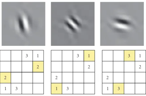
In the DDWT, different frequency tilings lead to different orientation of wavelets [10].Figure 15illustrates the orienta-tion of three subbands of isotropic 2D DDWT. The wavelets that have the subband indexed as 1, 2, and 3 have orienta-tions of approximately−45,−75, and−15 degrees as shown inFigure 15(for clarity, only 1 decomposition level is shown below).
Figure 16 demonstrates the 2D frequency tiling of
the isotropic and anisotropic wavelet transforms, respec-tively, for 2 levels of decomposition in each direction. In
Figure 16(b), the original LH and HL subbands are further
divided into two corresponding rectangular subbands. In
both Figures 16(a) and 16(b), wavelets that have the
sub-bands indexed as 1, 2, and 3 have orientation of approx-imately −45, −75, and −15 degrees. But in Figure 16(b), anisotropic wavelets corresponding to subbands 4 to 7 have some additional orientations of−81,−63,−9,−27 degrees.
1 2
3
1 2 3
1 2
3
1 2 3
1 2
3
1 2 3
Figure 15: Typical wavelets associated with the isotropic 2D DDWT. The top row illustrates the wavelets in the spatial domain, the second row illustrates the (idealized) support of the spectrum of each wavelet in the 2D frequency plane.
(Nr+ 1)(Nc+ 1)(Nt+ 1), whereNr,Nc, andNtare
decompo-sition levels for row, column, and temporal direction, respec-tively. Usually we use the same number of decomposition lev-els for the two special directions and allow different levels for the temporal direction. The additional subbands with diff er-ent orier-entations add to the flexibility of the original isotropic DDWT. Asides from the different decompositions within a single tree, all other implementations are just the same as DDWT [10], and the redundancy is not increased.
Figure 17demonstrates the structure of 3D isotropic and proposed anisotropic transforms in spacial and temporal do-mains. Both structures applied two wavelet decomposition levels. In the isotropic structure, only the low subband LLL is decomposed each time. But the anisotropic structure de-composes all subbands except the highest-frequency sub-band HHH into new subsub-bands. We applied noise shaping on the new anisotropic structure of 3D DDWT, and compared it to the original isotropic 3D DDWT and the standard 3D DWT. In this experiment, three wavelet decomposition levels are applied in each direction for both video sequences. The 3D DDWT and DWT filters are the same as inSection 2.
Figure 18shows that the 3D DDWT, both isotropic and
anisotropic structures, achieve better quality (in terms of PSNR) than the standard 3D DWT, with the same num-ber of retained coefficients. To achieve the same PSNR, the anisotropic structure needs about 20% fewer coefficients on average than the isotropic structure. With the same number of retained coefficients,DDWT NSyields higher PSNR than DWT. The anisotropic structure (DDWT anisotropic NS) outperforms the isotropic structure (DDWT isotropic NS) by 1-2 dB.
7.2. Combining 3D DDWT and DWT
The 3D DDWT isolates different spatial orientations and motion directions in each subband, which is desirable for video representations. In terms of 2D orientation, the DDWT is oriented along six directions: ±75◦, ±45◦, and
1 2
3
1 3
2 0
1 3
2 2 1 3
π
π
π π
(a) Isotropic tiling
1 5 4
7 6
1 3
2 0
5 1 3
2 4
1 7 6
π
π
π π
(b) Anisotropic tiling
Figure16: 2D anisotropic dual-tree wavelets for 2 levels of decom-position in each direction (from one tree).
±15◦. Unfortunately, the DDWT does not represent the
ver-tical and horizontal orientations (±0◦and±90◦) in pursuit
of other directions. Recognizing this deficiency, we propose to combine the 3D DDWT and DWT, to capture directions represented by both.
Considering that the horizontal and vertical orientations are usually dominant in natural video sequences, we gave the DWT priority to represent the video sequences. We as-sume that the horizontal and vertical features in the video sequences will be represented by large DWT coefficients. So we apply DWT at first and only keep the coefficients over a certain threshold. Then we apply the DDWT on the residual video, and the noise shaping is used to select the significant DDWT coefficients of the residual video. This is illustrated in
Figure 19. Recognizing that the DWT subband has a
normal-ized energy that is four times that of the DDWT subband, we use 1000 as the threshold for chosing significant 3D DWT co-efficients, and use 256 as the initial noise-shapping threshold for DDWT coefficients.
(a) Isotropic decomposition
(b) Anisotropic decomposition
Figure17: Comparison of isotropic decomposition and anisotropic decomposition.
than the 3D DDWT alone, with the same number of retained coefficients. To achieve the same PSNR, the combined trans-form needs up to 8% fewer coefficients than the 3D DDWT alone.
8. CONCLUSION
We demonstrated that the 3D DDWT has attractive proper-ties for video representation. Although the 3D DDWT is an overcomplete transform, the raw number of coefficients can be reduced substantially by applying noise shaping. The fact that noise shaping can reduce the number of coefficients to below that required by the DWT (for the same video qual-ity) is very encouraging. The vector entropy study validates our hypothesis that only a few basis functions have signifi-cant energy for an object feature. The relatively low vector entropy suggests that the whereabouts of significant coeffi -cients may be coded efficiently by applying vector arithmetic coding to the significance bits across subbands. The fact that coefficient values do not have strong correlation among the subbands, on the other hand, indicates that the benefit from vector coding the magnitude bits across the subbands may be limited.
Based on our investigation, two new video codecs, namely, DDWT-SPIHT and DDWTVC, using the 3D
dual-30 32 34 36 38 40 42
PSNR
(dB)
0.5 1 1.5 2
×106
Number of retained coefficients DDWT anisotropic NS
DDWT isotropic NS DWT
(a) Stefan (CIF)
30 32 34 36 38 40 42
PSNR
(dB)
0.5 1 1.5 2 2.5 3
×106
Number of retained coefficients DDWT anisotropic NS
DDWT isotropic NS DWT
(b) Mobile-Calendar (CIF)
Figure 18: Comparison of the reconstruction quality (in terms of PSNR) using the same number of retained coefficients with the isotropic DDWT with noise shaping (DDWT isotropic NS, upper curve) and the anisotropic DDWT with noise shaping (DDWT anisotropic NS, middle curve) and DWT (lower curve).
Video 3-D DWT Thresholding 3-D DWTInverse
3-D DDWT
−
Noise shaping Desired
coefficients
Figure19: The structure of combining 3D DDWT and DWT.
subband has not been explored in the current DDWTVC. Recognizing that context-based coding is an effective mean to explore such dependence, we have explored the use of context-based arithmetic vector coding. A main difficulty in applying context models is that the complexity grows expo-nentially with the number of pixels included in the context. We have tested the efficiency of various contexts, which differ in the chosen subbands and spatial neighbors. However the study so far has not yielded significant gain over direct vector coding.
Besides the standard isotropic decomposition structure, a new anisotropic structure of the novel 3D dual-tree wavelet transform is also proposed and tested on video coding. The anisotropic structure of the 3D DDWT decomposes not only the lowest subband LLL, but also all other subbands except the highest subband HHH. The number of the decomposi-tion stages can be different along temporal, horizontal, and vertical directions. This structure is more effective than the traditional isotropic structure. The anisotropic structure can yield better reconstruction quality (in terms of PSNR) for the same number of coefficients. We also propose to com-bine 3D DWT and DDWT to capture more directions and edges in video sequences. The combined structure, however, leads to only slight gains in terms of reconstruction quality versus number of coefficients.
In terms of future work, more properties of the 3D dual-tree transform need to be exploited. First of all, a codec that can exploit both interbands and intraband correlation in coding the significance bits is expected to provide signif-icant improvement. Secondly, how to incorporate the pro-posed anisotropic DDWT in video coding is still open, be-cause the number of subbands and orientations increases more dramatically in anisotropic structure. Based on the gain in terms of the reconstruction quality versus number of (unquantized) coefficients, we expect that a codec us-ing the anisotropic DDWT can lead to additional signifi-cant gains. The codec in [22] exploits both inter- and in-traband correlations. It also compares the performance ob-tainable with isotropic and anisotropic decomposition. With isotropic DDWT, their codec has, however, similar perfor-mance as DDWTVC. The anisotropic DDWT achieved on average a gain of 1 dB over isotropic. Finally, with noise shap-ing, the optimal set of coefficients to be retained changes with the target bit rate. To design a scalable video coder, we would like to have a scalable set of coefficients so that each addi-tional coefficient offers a maximum reduction in distortion without modifying the previous coefficients. How to deduce such coefficient sets is a challenging open research problem.
30 32 34 36 38 40
PSNR
(dB)
4 6 8 10 12 14
Number of retained coefficients ×105 DDWT NS
DDWT DWT NS
(a) Stefan (CIF)
29 30 31 32 33 34 35 36 37
PSNR
(dB)
4 6 8 10 12
Number of retained coefficients ×105 DDWT NS
DDWT DWT NS
(b) Mobile-Calendar (CIF)
Figure 20: Comparison of the reconstruction quality (in terms of PSNR) using the same number of retained coefficients with DDWT (DDWT NS, upper curve) and the combined DDWT and DWT(DDWT DWT NS, lower curve). The DDWT coefficients are obtained by noise shaping in both cases.
ACKNOWLEDGMENTS
REFERENCES
[1] S.-T. Hsiang and J. W. Woods, “Embedded video coding us-ing invertible motion compensated 3-D subband/wavelet filter bank,”Signal Processing: Image Communication, vol. 16, no. 8, pp. 705–724, 2001.
[2] J. Xu, Z. Xiong, S. Li, and Y.-Q. Zhang, “Memory-constrained 3-D wavelet transform for video coding without boundary effects,”IEEE Transactions on Circuits and Systems for Video Technology, vol. 12, no. 9, pp. 812–818, 2002.
[3] Y. Andreopoulos, M. van der Schaar, A. Munteanu, J. Bar-barien, P. Schelkens, and J. Cornelis, “Fully-scalable wavelet video coding using in-band motion compensated temporal fil-tering,” inProceedings of IEEE International Conference on Ac-coustics, Speech, and Signal Processing (ICASSP ’03), vol. 3, pp. 417–420, Hong Kong, April 2003.
[4] A. Secker and D. Taubman, “Lifting-based invertible motion adaptive transform (LIMAT) framework for highly scalable video compression,”IEEE Transactions on Image Processing, vol. 12, no. 12, pp. 1530–1542, 2003.
[5] “Joint Scalable Video Model 2.0 Reference Encoding Al-gorithm Description,” ISO/IEC JTC1/SC29/WG11/N7084. Buzan, Korea, April 2005.
[6] N. Kingsbury, “A dual-tree complex wavelet transform with improved orthogonality and symmetry properties,” in Pro-ceedings of IEEE International Conference on Image Process-ing (ICIP ’00), vol. 2, pp. 375–378, Vancouver, BC, Canada, September 2000.
[7] M. N. Do and M. Vetterli, “The contourlet transform: an effi -cient directional multiresolution image representation,”IEEE Transactions on Image Processing, vol. 14, no. 12, pp. 2091– 2106, 2005.
[8] T. H. Reeves and N. G. Kingsbury, “Overcomplete image cod-ing uscod-ing iterative projection-based noise shapcod-ing,” in Proceed-ings of IEEE International Conference on Image Processing (ICIP ’02), vol. 3, pp. 597–600, Rochester, NY, USA, September 2002. [9] K. Sivaramakrishnan and T. Nguyen, “A uniform transform domain video codec based on dual tree complex wavelet transform,” inProceedings of IEEE International Conference on Acoustics, Speech and Signal Processing (ICASSP ’01), vol. 3, pp. 1821–1824, Salt Lake City, Utah, USA, May 2001.
[10] I. Selesnick and K. Y. Li, “Video denoising using 2D and 3D dual-tree complex wavelet transforms,” inWavelets: Applica-tions in Signal and Image Processing X, vol. 5207 ofProceedings of SPIE, pp. 607–618, San Diego, Calif, USA, August 2003. [11] I. Selesnick, R. G. Baraniuk, and N. C. Kingsbury, “The
dual-tree complex wavelet transform,”IEEE Signal Processing Mag-azine, vol. 22, no. 6, pp. 123–151, 2005.
[12] B. Wang, Y. Wang, I. Selesnick, and A. Vetro, “An investi-gation of 3D dual-tree wavelet transform for video coding,” inProceedings of International Conference on Image Processing (ICIP ’04), vol. 2, pp. 1317–1320, Singapore, October 2004. [13] B.-J. Kim, Z. Xiong, and W. A. Pearlman, “Low bit-rate
scal-able video coding with 3-D set partitioning in hierarchical trees (3-D SPIHT),”IEEE Transactions on Circuits and Systems for Video Technology, vol. 10, no. 8, pp. 1374–1387, 2000. [14] B. Wang, Y. Wang, I. Selesnick, and A. Vetro, “Video coding
using 3-D dual-tree discrete wavelet transforms,” in Proceed-ings of IEEE International Conference on Acoustics, Speech and Signal Processing (ICASSP ’05), vol. 2, pp. 61–64, Philadelphia, Pa, USA, March 2005.
[15] D. Xu and M. N. Do, “Anisotropic 2D wavelet packets and rect-angular tiling: theory and algorithms,” inWavelets: Applica-tions in Signal and Image Processing X, vol. 5207 ofProceedings of SPIE, pp. 619–630, San Diego, Calif, USA, August 2003. [16] D. Xu and M. N. Do, “On the number of rectangular tilings,”
IEEE Transactions on Image Processing, vol. 15, no. 10, pp. 3225–3230, 2006.
[17] S. G. Mallat and Z. Zhang, “Matching pursuits with time-frequency dictionaries,”IEEE Transactions on Signal Process-ing, vol. 41, no. 12, pp. 3397–3415, 1993.
[18] R. Gribonval and P. Vandergheynst, “On the exponential con-vergence of matching pursuits in quasi-incoherent dictionar-ies,”IEEE Transactions on Information Theory, vol. 52, no. 1, pp. 255–261, 2006.
[19] R. Neffand A. Zakhor, “Very low bit-rate video coding based on matching pursuits,”IEEE Transactions on Circuits and Sys-tems for Video Technology, vol. 7, no. 1, pp. 158–171, 1997. [20] H. Bolcskei and F. Hlawatsch, “Oversampled filter banks:
opti-mal noise shaping, design freedom, and noise analysis,” in Pro-ceedings of IEEE International Conference on Acoustics, Speech and Signal Processing (ICASSP ’97), vol. 3, pp. 2453–2456, Mu-nich, Germany, April 1997.
[21] J. Hua, Z. Xiong, and X. Wu, “High-performance 3-D embed-ded wavelet video (EWV) coding,” inProceedings of 4th IEEE Workshop on Multimedia Signal Processing (MMSP ’01), pp. 569–574, Cannes, France, October 2001.