Pseudodynamic tests and earthquake response analysis of timber structures III: three-dimensional conventional wooden structures with plywood-sheathed shear walls

(1)

ORIGINAL ARTICLE

Takahisa Kamada · Motoi Yasumura · Shimpei Yasui Luc Davenne · Motoi Uesugi

Pseudodynamic tests and earthquake response analysis of timber

structures III: three-dimensional conventional wooden structures with

plywood-sheathed shear walls

Abstract Pseudodynamic (PSD) tests were conducted on plywood-sheathed conventional Japanese three-dimensional (3D) wooden structures. Lateral load was applied to the edge beam of specimen structures to generate eccentricity loading. Specimens were based on a combination of shear walls with openings in the loading direction and horizontal diaphragms with different shear stiffness. The principle deformation of the horizontal diaphragm was torsion for rigid diaphragms and shear deformation for fl exible dia-phragms. Lumped-mass time-history earthquake response analysis was conducted on the tested structures, and addi-tional calculations were conducted on structures with differ-ent eccdiffer-entricity rates. Dynamic analyses were conducted by varying the masses and the resistance of the walls in the loading direction. The simulated peak displacement response in the loading plane agreed comparatively well with the PSD test results. The maximum displacement response on chang-ing the wall resistant ratio showed almost the same tendency as that obtained by changing the mass ratio up to an eccen-tricity rate of 0.3; however, the maximum displacement response increased markedly beyond an eccentricity rate of 0.4. It was proved that the lumped-mass 3D model proposed

in this study was appropriate for conducting a parameter study on the 3D dynamic behavior of timber structures.

Key words Computer online control · Lumped-mass model · Dynamic analysis · 3D Structures · Plywood sheathing

Introduction

The infl uence of eccentricity wall layout and mass distribution on the seismic performance of timber structures is of rele-vance to the design of timber structures. A number of experi-mental and theoretical studies have been conducted on this subject, but few have dealt with the infl uence of the in-plane shear stiffness on the seismic behavior of timber structures. Therefore, it is of great importance to develop a comparatively simple method to predict the behavior of three-dimensional (3D) structures and to validate this method by a simplifi ed testing method. We consider that pseudodynamic (PSD) testing is an appropriate method for this purpose as this test method requires relatively simple apparatus and measuring system comparing to shake-table tests.1–3

In this study, small 3D structures were subjected to eccentricity pseudodynamic loads simulating the seismic response, and the experimental results were compared with the results of time history earth-quake response analysis including a shear stiffness matrix for the horizontal diaphragm and the lumped-mass model for the shear walls. The hysteresis model of shear walls proposed in previous studies4–6

was applied to the simulation, and the pseudodynamic test results showed that the 3D model pro-posed in this study predicted well the three-dimensional behavior of timber structures with either a rigid or fl exible horizontal diaphragm.

Specimens

Japanese conventional post and beam structures with plywood-sheathed shear walls and a horizontal diaphragm

Received: February 20, 2011 / Accepted: April 15, 2011 / Published online: August 2, 2011 DOI 10.1007/s10086-011-1198-6

T. Kamada (*)

United Graduate School of Agricultural Science, Gifu University, 836 Ohya, Suruga-ku, Shizuoka 422-8529, Japan

Tel. +81-54-237-1111; Fax +81-54-237-3028 e-mail: [email protected] M. Yasumura

Faculty of Agriculture, Shizuoka University, Shizuoka 422-8529, Japan S. Yasui

Research and Development Center, DAIKEN Corporation, Okayama 702-8045, Japan

L. Davenne

Laboratoire de Mecanique et Technologie, ENS Cachan, 94235 Cachan, France

M. Uesugi

Miyazaki Prefecture Wood Utilization Research Center, Miyakonojo, Miyazaki 885-0037, Japan

(2)

were prepared for the PSD tests. Figure 1 gives a general depiction of the specimen and test setup. Specimens had the shape of a cube 3 m on an edge. Posts, sills, and joists were 105 × 105-mm spruce (Picea spp.) glued laminated timber complying with JAS E85-F300, and beams were 105 × 210-mm spruce glued laminated timber complying with JAS E95-F270. Studs and headers were 30 × 105-mm and 45 × 10-mm spruce lumber, respectively. Posts placed every 1000 mm were connected to the sill and beam with a steel pipe of 26.5 mm diameter and hold-down connections.7 Studs placed at the center between posts were fastened to the sill and beam with two N75 nails at both ends of the studs. Joists were connected to the beam by metal joist hangers spaced 1000 mm apart. Each sill was anchored to the steel base frame with three M16 bolts positioned at the center and 150 mm inside from the ends. Seven-and-a-half-millimeter-thick, 1000-mm-wide, and 3000-mm-long lauan plywood of JAS Grade 18 with a density of 880 kg/m3 was sheathed on the wall frames with N50 nails at intervals of 150 mm.

Walls parallel to the loading direction in the X1 and X2 planes had an opening of window confi guration (1 m wide and 1 m height) (W) or an opening 1 m wide and 3 m high at the center of the wall (S), as shown in Fig. 2; walls per-pendicular to the loading direction in the Y1 and Y2 planes had no openings. Specimen WW had walls W on both X1

and X2 planes, and specimen WS had a wall W in the X1 plane and a wall S on the X2 plane. Figure 3 shows the details of the horizontal diaphragm. A horizontal diaphragm of 3 × 3 m2

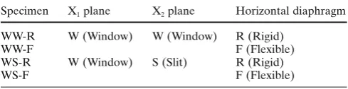
consisted of 105 × 210-mm beams and 105 × 105-mm joists spaced 1000 mm apart. Twenty-four-millimeter-thick sugi plywood of JAS Grade 2, 1000 mm wide and 2000 mm long, was sheathed on the fl oor frame with N75 nails at intervals of 150 mm. Two kinds of dia-phragm with different in-plane shear stiffness were pre-pared. A rigid horizontal diaphragm (R) in which all the edges of the plywood sheathing were nailed to the beams, joists, and 60 × 60-mm bridging joists placed at the plywood joints was prepared to provide comparatively high shear stiffness, and a fl exible diaphragm (F) in which all nails on the longitudinal edges of the plywood were omitted was expected to have a lower shear stiffness. Table 1 summarizes the specimens based on the combination of wall types in the X1 and X2 planes and horizontal diaphragms of different shear stiffness.

Test methods

Racking test of the horizontal diaphragm

Racking tests of the horizontal diagram were conducted to determine the parameters for modeling the load– displacement relationships. The same types of fl oor (R and F) were prepared, except that the beam sections were reduced to 105 × 105 mm. The loading protocol used for the reversed cyclic tests was based on the international standard

Fig. 1. Confi guration of the specimen structure

1000

3000

1000

Window (W)

0

10

0

1

1000

1000 1000 1000 1000

Slit (S)

(mm)

Fig. 2. Confi guration of window (W) wall and slit (S) wall

1m

Flexible (F)

Rigid (R)

X Y

2m 1m

Fig. 3. Frame and nail patterns for rigid (R) and fl exible (F)

dia-phragms. In rigid diaphragms, sheets are nailed on beams, joists, and bridging joists; in fl exible diaphragms, sheets are not nailed on beams or bridging joists

Table 1. Specimen structures that underwent pseudodynamic testing

Specimen X1 plane X2 plane Horizontal diaphragm

WW-R W (Window) W (Window) R (Rigid)

WW-F F (Flexible)

WS-R W (Window) S (Slit) R (Rigid)

(3)

ISO 21581.9

The lateral load was measured by a load cell (capacity: ±50 kN, Tokyo Sokki Kenkyujo, Tokyo) and the horizontal displacements at the corner of the diaphragm were measured by electronic transducers (capacity: 100 mm, Tokyo Sokki Kenkyujo, Tokyo).

Lateral loading tests of 3D structures

Specimen structures were anchored on the steel base frame, which was tightly connected to the reinforced concrete reac-tion fl oor, and the lateral load was applied to the edge beam of the specimen by an actuator that was connected to the reinforced concrete reaction wall with a pin joint. Four sills of the specimen were anchored to the steel base frame with three M16 bolts positioned at the center and 150 mm inside from the ends, and an actuator was connected to the end of the X1 plane with a pin joint, as shown in Fig. 1. The reason why the lateral load was applied at the edge beam instead of the center of the specimen was to observe more clearly the effects of the shear stiffness of the horizontal diaphragm on the seismic behavior of the 3D structure. Dynamic analy-sis, as described later, with and without eccentricity mass distribution and wall stiffness was conducted to follow up the test results.

The PSD tests were conducted by using a computer online system (Saginomiya ATC-20). Horizontal displace-ments were applied at the edge beam of the structure step by step by resolving the differential equation based on the displacement and the reaction force obtained at the previ-ous step. The mass and the damping factor were assumed to be 10 tonne (t) and 2%, respectively, for all specimens. The accelerogram used for the PSD tests was the 1940 El Centro NS and the maximum acceleration was scaled up to 0.4 g. Horizontal displacements in the X and Y directions at the top of the specimen and the vertical displacements of each post were measured by electric transducers.

Experimental results

Horizontal diaphragm

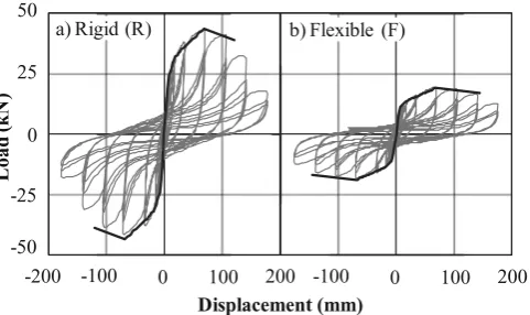
Figure 4 shows the relationship between the lateral load and displacement of the horizontal diaphragm in cyclic tests with fl exible (F) and rigid (R) diaphragms. The stiffness, yield, and ultimate loads obtained from the Japan Housing and Wood Technology Center guidelines for conventional wooden construction10

were 3.39 kN/mm, 24.21 kN, and 39.00 kN for the rigid diaphragm (R) and 1.72 kN/mm, 11.08 kN, and 17.03 kN for the fl exible diaphragm (F), respectively. The latter were 0.51, 0.46, and 0.44 times those of the former, indicating that the stiffness and the bearing capacity decrease rapidly when the nail joints in the longi-tudinal edge of the fl oor sheeting were removed.

3D structures

Figure 5 shows the time–displacement response relation-ships under PSD testing. Table 2 shows the maximum

-200 0 200

-50 50

0 25

-25

-100 100

L

oad (

k

N

)

Displacement (mm) a) Rigid (R)

200 0

-100 100

b) Flexible (F)

Fig. 4. Load–displacement relationship in cyclic tests for a the rigid

diaphragm (R) and b the fl exible diaphragm (F). The bold line repre-sents the backbone curve

Fig. 5. Time–displacement

response relationships under pseudodynamic (PSD) testing.

Black solid lines, gray solid lines, black dotted lines, and gray dotted lines represent the X1, X2,

Y1, and Y2 planes, respectively

0

2.5

5.0

7.5

10 0

2.5

5.0

7.5

10

Time (s)

Displacement response (mm)

-100

0

100

-100

0

100

WW-R

WW-F

WS-R

WS-F

(4)

q

_y

=

d

_y

/ L

x

y

γ

d

_x

L

H

q

x

=

d

x

/ H

g

=

|

q

x

-

q

y

|

d

_y

q

y

q

x

Fig. 6. Defi nition of θx, θy, and shear deformation angle γ

m

x1

m

_x₂

X

1

k

x1

X

₂

k

_x₂

m

y

1

Y

1

k

y1

m

y

2

Y

2

k

y2

G

_f

L

H

Fig. 7. Plan view of the lumped-mass model for a three-dimensional

specimen

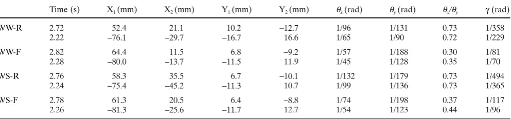
displacement responses in the X1 plane in the positive and negative directions and those of other planes when the dis-placement in the X1 plane was maximum; the defi nitions of

θx, θy, and the shear deformation angle γ are shown in Fig. 6. Specimens with rigid diaphragms (WW-R, WS-R) and fl exible diaphragms (WW-F, WS-F) showed almost the same maximum displacement response at the X1 plane. However, the average maximum displacement response in the posi-tive and negaposi-tive directions at the X2 plane of specimens WW-R and WS-R were 40% and 60% of those at the X1 plane, respectively, and the maximum displacement response at the X2 plane of specimens WW-F and WS-F were 17% and 32% of those at the X1 plane, respectively. The shear deformation angles of the horizontal diaphragm for WW-R and WS-R were 1/229 rad and 1/365 rad, and those of speci-mens WW-F and WS-F were 1/70 rad and 1/96 rad, respec-tively. The ratios of θx to θy of the horizontal diaphragm of specimens WW-R and WS-R were 0.72 and 0.73 on an average for positive and negative displacements, and those of specimens WW-F and WS-F were 0.33 and 0.40, respectively.

This indicates that the shear force transmission from the X1 plane to the X2 plane decreased considerably when the nail joints in the longitudinal edge of fl oor sheathing were removed. Therefore, the principle deformation of the rigid

diaphragm (R) is torsion, while the principle deformation of the fl exible diaphragm (F) is shear deformation.

Dynamic analysis

Modeling of 3D structures

A lumped-mass model with nonlinear springs, as shown in Fig. 7, was assumed for the dynamic analysis. The model consisted of four masses (mx1, mx2, my1, and my2) supported by four nonlinear springs (kx1, kx2, ky1, and ky2) that represent the four vertical walls. These masses are connected to each other with a stiffness matrix representing the horizontal diaphragm. It was assumed that the horizontal diaphragm deforms as a parallelogram and has linear shear stiffness of Gf. The stiffness matrix for the horizontal diaphragm Kf is expressed as follows:

Table 2. Displacement response of each plane and the horizontal diaphragm deformation angles θx, θy, and γ when the displacement of the X1

plane was at maximum

Time (s) X1 (mm) X2 (mm) Y1 (mm) Y2 (mm) θx (rad) θy (rad) θx/θy γ (rad)

WW-R 2.72 52.4 21.1 10.2 −12.7 1/96 1/131 0.73 1/358 2.22 −76.1 −29.7 −16.7 16.6 1/65 1/90 0.72 1/229 WW-F 2.82 64.4 11.5 6.8 −9.2 1/57 1/188 0.30 1/81

2.28 −80.0 −13.7 −11.5 11.9 1/45 1/128 0.35 1/70 WS-R 2.76 58.3 35.5 6.7 −10.1 1/132 1/179 0.73 1/494

(5)

K G L H L H L H L H H L H L H L H L f= f×

− − − − − − − − ⎡ ⎣ ⎢ ⎢ ⎢ ⎢ ⎢ ⎢ ⎢ ⎢ ⎤ ⎦ ⎥ ⎥ ⎥ ⎥ ⎥ ⎥ ⎥ ⎥ 1 1 1 1 1 1 1 1

where Gf is the shear stiffness of the diaphragm and L and H are the length and depth of the diaphragm, respec-tively.11–14

Shear walls composing the structure were modeled with the hysteresis model proposed in previous studies,4,5,15 including Foschi’s model16 for the backbone curves and the slip model for unloading and reloading, as shown in Fig. 8. The model is defi ned by the following expressions:

P₌ P ₊C x ₋e−C×x P

( 0 2 )(1 1 0) (1)

P=Pm−C x3 −Dm (2)

k k1 =C4×X Cm 5+1 (3)

k k2 0= −1 C X6 m−X C0 7 (4)

k k3 =C8×X Cm 9+1 (5)

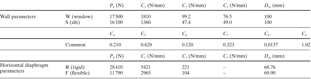
Table 3. Hysteresis parameters of wall hysteresis and horizontal diaphragms for use in Eqs. 1–5

P0 (N) C1 (N/mm) C2 (N/mm) C3 (N/mm) Dm (mm) Wall parameters W (window) 17 500 1810 99.2 76.5 100

S (slit) 16 100 1360 47.4 49.0 100

C4 C5 C6 C7 C8 C9

Common 0.210 0.628 0.120 0.323 0.0137 1.02

P0 (N) C1 (N/mm) C2 (N/mm) C3 (N/mm) Dm (mm)

Horizontal diaphragm

parameters R (rigid)_{F (fl exible)} 28 410_{11 790} 5421₂₉₆₅ 221₁₀₄ –_– 68.76_69.90 The wall parameters are quoted from Yasumura and Yasui5

The values of C4–C9 were the same for both types of wall

Fig. 8. Hysteresis model of shear walls. Numbers in parentheses

cor-respond to the equation number in the text: (1) loading on the back-bone curve up to the maximum load, (2) loading on the backback-bone curve above the maximum load, (3) unloading from the peak on the back-bone curve, (4) reloading with a soft spring, (5) reloading toward the previous peak with a hard spring

(1)

(2)

(3)

(4)

(5)

k

₁

k

₃

k

₂

k

₀

(X

m

,Y

m

)

(D

m

,P

m

)

(D

u

,0.8P

m

)

X (D)

Y (P)

Parameters obtained from the racking tests of shear walls with openings in the previous study were applied to the dynamic analysis of the structures. Backbone curves of the horizontal diaphragm were also modeled with Foschi’s model; however the load–displacement relation was assumed to be linear, the slope of which was defi ned by the point on the backbone curve with the maximum displace-ment ever experienced. The model parameters P0, C1, C2, and C3 were obtained from the racking test of the horizontal diaphragm as shown in Table 3.

Time history earthquake response analysis

Lumped-mass time-history earthquake response analysis was conducted on the tested structures. The mass mx1 was set at 10 t, and the other masses mx2, my1, and my2 were assumed to be almost zero. The same accelerogram as used in the PSD tests, 1940 El Centro NS scaled up to 0.4 g , was applied to the dynamic analysis. The damping factor was set at 2%. Additional calculations with different eccentricities were conducted to follow up the test results.

First, the dynamic analyses were conducted on specimen WW and specimen WS with the same conditions as the former analysis by varying the masses mx1 and mx2 from 0 to 10 t, respectively, so that the sum of mx1 and mx2 was kept at 10 t. In this procedure, the eccentricity rate10

of specimens WW and WS varied from 0 to 0.81 and from 0 to 0.73, respectively.

Second, dynamic analysis was conducted on specimen WW with masses mx1 and mx2 kept at 5 t each and the resis-tance factor of the walls in the X1 and X2 planes varied from 15% to 185% of the original wall (W) so that the sum of the stiffness and resistance of walls in the X1 and X2 planes was twice those of wall (W). In this procedure, the eccentric-ity rate varied from 0 to 0.52.

Results and discussion

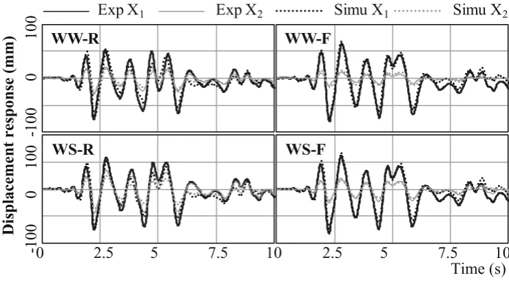
Comparison of simulation with experimental results

(6)

0

2.5

5

7.5

10

2.5

5

7.5

10

Time (s)

-100

0

100

-100

0

100

WW-R

WW-F

WS-R

WS-F

Exp X

1

Exp X

2

Simu X

1

Simu X

2

Fig. 9. Displacement responses

at the X1 and X2 planes in the

PSD tests and simulation results.

Black solid lines and gray solid lines are the experimental results

for the X1 and X2 planes,

respectively. Black dotted lines and gray dotted lines are the simulation results for the X1 and

X2 planes, respectively

Table 4. Displacement response of each plane and the horizontal diaphragm deformation angle γ when the displacement of the X1 plane was at

maximum for structure WW-R

Time (s) X1 (mm) X2 (mm) Y1 (mm) Y2 (mm) γ (rad)

Positive

Experiment 2.72 52.4 21.1 10.2 −12.7 1/358 Simulation 2.76 51.6 19.2 11.9 −11.9 1/347

Ratio 1.02 1.10 0.86 1.07 0.97

Negative

Experiment 2.22 −76.1 −29.7 −16.7 16.6 1/229 Simulation 2.26 −71.3 −26.5 −17.4 17.4 1/304

Ratio 1.07 1.12 0.96 0.95 1.33

Table 5. Displacement response of each plane and the horizontal diaphragm deformation angle γ when the displacement of the X1 plane was

at maximum for structure WW-F

Positive

Ratio 0.94 0.80 0.80 1.08 0.99

Negative

Ratio 1.06 0.85 1.19 1.23 1.07

at maximum for structure WS-R

Positive

Ratio 1.11 1.49 0.65 0.98 0.75

Negative

(7)

at maximum for structure WS-F

Positive

Ratio 0.91 1.17 0.77 1.06 0.77

Negative

Ratio 1.09 1.25 1.26 1.36 0.88

indicates that the simulation agreed comparatively well with the PSD test results. Tables 4–7 shows that the displace-ment responses of the X1, X2, Y1, and Y2 planes at the time of peak displacement response agreed comparatively well with the PSD test results, except for WS-R.

In specimen WS-R, the ratios of positive (tensile) peak displacement responses in the PSD test to simulations in the X2 and Y1 planes were 1.49 and 0.65, respectively. The dis-tinction between the experimental results and simulation results was as large as 35%–49%. It is supposed that the torsional displacement might be restrained by the tensile force applied at the end of the edge beam.

Figure 10 shows the deformation of the horizontal dia-phragm in the PSD tests and the simulation at the time of the peak displacement in the X1 plane, as shown in Tables 4–7. The horizontal displacements in the X and Y directions are magnifi ed by a factor of ten. It is noted that the

simula-1500mm

1500m

m

WW-R

WW-F

WS-R

WS-F

Fig. 10. Deformation of the horizontal diaphragm in the PSD tests and

the simulation results. The deformation in the X and Y directions are magnifi ed by ten. Gray lines indicate experimental results and black

lines indicate the simulation results

X1 (W)

X2 (W)

X1 (W)

WW-R:Exp

WW-F:Exp

m-(WW-R):Simu

m-(WW-F):Simu

(W) Wall:Exp

0 0.2

0.4

0.6

0.8

1.0

eccentricity rate

120

90

60

30

0

-30

-60

-90

-120

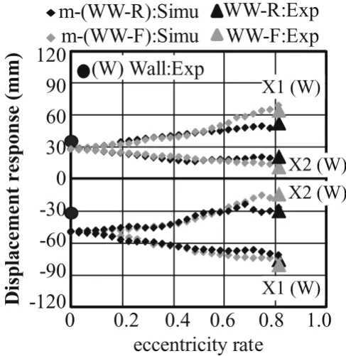
Fig. 11. Maximum displacement response–eccentricity rate

relation-ship, where m-(WW-R) and m-(WW-F) are the displacement responses in the simulation in which the mass ratio between the X1 and X2 planes

varied. Triangles indicate PSD test results of specimens WW-R and WW-F, circles indicate the PSD test results of wall W from Yasumura and Yasui5

tion predicts quite well the deformation of the horizontal diaphragm in the PSD tests.

Infl uence of the eccentricity on the earthquake response

(8)

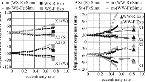
Fig. 12. Maximum displacement response–eccentricity rate

relation-ship, where m-(WS-R) and m-(WS-F) are the same as indicated in Fig. 11. Squares represent the PSD test results of specimens WS-R and WS-F

0 0.2

0.4

0.6

0.8

1.0

eccentricity rate

X1 (W)

120

90

60

30

0

-30

-60

-90

-120

X2 (S)

X1 (W)

WS-R:Exp

WS-F:Exp

m-(WS-R):Simu

m-(WS-F):Simu

0 0.2

0.4

0.6

0.8

1.0

m-(WW-R):Simu

m-(WW-F):Simu

St-(R):Simu

St-(F):Simu

WW-R:Exp

WW-F:Exp

eccentricity rate

120

90

60

30

0

-30

-60

-90

-120

X1

X2

X1

Fig. 13. Maximum displacement response–eccentricity rate

relation-ship, where St-(R) and St-(F) stand for displacement responses in the simulation in which the wall resistance between the X1 and X2 planes

varied

in the X1 plane to that of the X2 plane was greater than 2 when the eccentricity rates of specimens WW-R, WW-S, WS-R, and WS-S were 0.36, 0.45, 0.41, and 0.47, respectively. The ratio of maximum displacement response in specimen WW with a fl exible diaphragm (F) to that of the specimen with a rigid diaphragm (R) was at most 1.37, which occurred when the mass was positioned at one edge of the specimen.

Figure 13 shows the relationship between the eccentric-ity rate and maximum displacement response, together with the results as shown in Fig. 11, when the wall resistant ratio at the X2 plane to that of the X1 plane varied from 1.0 to 12.33. The maximum displacement response by changing the wall resistant ratio showed almost the same tendency as that obtained by changing the mass ratio up to an eccentric-ity rate of 0.3; however, the maximum displacement response increased markedly beyond an eccentricity rate of 0.4.

Conclusions

The results obtained in this study can be summarized as follows. Pseudodynamic (PSD) tests showed that the shear force transmission from the X1 plane to the X2 plane decreased considerably when the nails in the longitudinal edge of the fl oor sheathing were removed. Therefore, the principle deformation of the rigid diaphragm (R) was torsion, while that of the fl exible diaphragm (F) was shear deformation. The simulated values of the displacement responses of the X1, X2, Y1, and Y2 planes at the time of peak

displacement response of the X1 plane agreed well with the PSD test results. The ratio of the maximum displacement responses in the X1 plane to that of the X2 plane was greater than 2 when the eccentricity rate of specimens WW-R, WW-S, WS-R, and WS-S were 0.36, 0.45, 0.41, and 0.47, respectively. The ratio of maximum displacement response in a WW structure with a fl exible diaphragm (F) to that with a rigid diaphragm (R) was at most 1.37 and occurred when the mass was located at one edge of the specimen. The maximum displacement response on changing the wall resistant ratio showed almost the same tendency as that obtained by changing the mass ratio up to an eccentricity rate of 0.3; however, the maximum displacement response increased markedly beyond an eccentricity rate of 0.4. The simulation predicted quite well the earthquake responses of the structures. The lumped-mass 3D model proposed in this study is suitable for conducting a parameter study on the 3D dynamic behavior of timber structures.

Acknowledgments The authors appreciate fi nancial support of the

Grants-in-Aid for Scientifi c Research “Category C” Monbu Kagakusho and JSPS.

References

1. Shing PB, Nakashima M, Bursi OS (1996) Application of pseudo-dynamic test method to structural research. Earthq Spectra 12:29–56

(9)

3. Kawai N (1998) Pseudo-dynamic test on shear walls. In: Proceed-ings of the 5th WCTE, vol 1, August, 1998, EPF Lausanne, Montreux, Switzerland, pp 412–419

4. Yasumura M (2001) Evaluation of damping capacity of timber structures for seismic design. In: Proceedings of the 34th CIB-W18, Venice, Italy, paper 34-15-3, pp 1–9

5. Yasumura M, Yasui S (2006) Pseudodynamic tests and earthquake response analysis of timber structures I: plywood-sheathed conven-tional wooden walls with opening. J Wood Sci 52:63–68

6. Yasumura M, Kamada T, Iimura Y, Uesugi M, Daudeville L (2006) Pseudodynamic tests and earthquake response analysis of timber structures II: two-level conventional wooden structures with plywood sheathed shear walls. J Wood Sci 52:69–74

7. Japan Housing and Wood Technology Center (2003) The testing method of metal fastenings and fasteners for wooden construction (in Japanese). Japan Housing and Wood Technology Center, Tokyo 8. Japan Agricultural Standard (2008) JAS for plywood (in Japanese).

JAS, Tokyo

9. ISO (2010) ISO 21581–2010: timber structures – static and cyclic lateral load test method for shear walls. ISO, Geneva

10. Japan Housing and Wood Technology Center (2001) Allowable strength design for Japanese conventional construction (in Japa-nese). Japan Housing and Wood Technology Center, Tokyo

11. Richard N, Yasumura M, Davenne L (2003) Prediction of seismic behavior of wood-framed shear walls with openings by pseudody-namic test and FE model. J Wood Sci 49:145–151

12. Yasumura M, Uesugi M, Luc D (2006) Estimating 3D behaviour of conventional timber structures with shear walls by pseudo-dynamic test. In: Proceedings of the 37th CIB-W18, August 30–Septmeber 3, Edinburgh, Scotland

13. Richard N, Yasumura M (2008) Dynamic model for 3D timber structures with plywood sheathed shear walls. In: Proceedings of the 10th WCTE, June 2–5, Miyazaki, Japan

14. Yasumura M, Nicolas R, Luc D, Uesugi M (2006) Estimating seismic performance of timber structures with plywood-sheathed walls by pseudo-dynamic tests and time-history earthquake response analysis. In: Proceedings of the 9th WCTE, August 6–10, Portland, OR, USA

15. Yasumura M (2003) Pseudo-dynamic tests on conventional timber structures with shear walls. In: Proceedings of the 36th CIB-W18, August 11–14, Colorado, USA