3D Soft Body Simulation Using Mass-spring System with Internal Pressure Force and Simplified Implicit Integration

3D Soft Body Simulation Using Mass-spring

System with Internal Pressure Force and

Simplified Implicit Integration

Jaruwan Mesit, Ratan Guha and Shafaq Chaudhry

School of Electrical Engineering and Computer Science, University of Central Florida, Orlando, Florida 32816 Email: {jmesit, guha, shafaq}@eecs.ucf.edu

Abstract— In this paper, we propose a method to simulate soft bodies by using gravitational force, spring and damping forces between surface points, and internal molecular pressure forces. We consider a 3D soft body model composed of mesh points that define the body’s surface such that the points are connected by springs and influenced by internal molecular pressure forces. These pressure forces have been modeled on gaseous molecular interactions. Simulation of soft body with internal pressure forces is known to become unstable when high constants are used and is averted using an implicit integration method. We propose an approximation to this implicit integration method that considerably reduces the number of computations in the algorithm. Our results show that the proposed method realistically simulates soft bodies and improves performance of the implicit integration method.

Index Terms— Soft body simulation, implicit integration method, internal pressure force, mass-spring system

I. INTRODUCTION

Soft body models simulate real-world objects that deform as they interact with the environment, e.g., clothes, hair, sand, and liquids [12, 15, 16, 17, 18, 22, 29, 30]. A body object is modeled by a group of points, each of which has properties such as position, velocity, force, etc. During each animation time step, the surface points get rearranged into new positions and their properties change, due to external interaction with the environment, and internal characteristics of the model itself.

Extensive research has been conducted on modeling and simulating soft bodies. Complex physics-based models have been developed for accurate and realistic soft body deformations that involve a high number of computations. These include finite element method (FEM) [2, 6, 7, 11], finite volume method (FVM) [1, 2], and long element method (LEM) [8, 9, 10]. On the other hand, there are models based on mass-spring system [20, 21, 28] that provide approximate deformation behavior, yet, are intuitively simple and execute much faster than accurate models. There are, however, some drawbacks in mass-spring systems [13]. The spring connections between points are not easily derived from measured material properties. Moreover, a mass-spring system with explicit integration cannot handle increased stiffness under large spring constants. Stiffness in a system causes

poor stability and requires the numerical integrator to take small time steps, even when the results of motion occur over much larger time intervals. These problems have been addressed by Desbrun et al. [14] and Kang et al. [19] who have proposed efficient and stable algorithms for animating a mass-spring system with the latter offering a faster calculation. In general, the implicit methods require more memory resources and high number of computations since they involve unknown values.

In this paper, we propose and present an implicit integration method for animating soft bodies. We model surface of the soft body by using a mass-spring system and simulate internal characteristics of the soft body using pressure forces. To show that our proposed method solves the stiffness problem, we compare it with the explicit integration method. Moreover, we provide a performance comparison between the explicit integration method, an adapted version of the implicit integration method presented in [19], and our proposed method. The results show that motion of soft bodies can be realistically rendered with the proposed implicit method, even with large spring constants.

The paper proceeds as follows: Section II provides some background on soft body simulation, and Section III details our approximated implicit method. In Section IV, we present the explicit and implicit methods with which we compare our proposed simplified implicit method. Section V presents the simulation experiments and comparison results. In Section VI, we cite applications that can be implemented by the proposed method. Finally, we conclude in Section VII, and discuss possible further work.

II. BACKGROUND

A. Mass-spring System to Model a Soft Body

Soft bodies using mass-spring systems can be classified into two different categories: modeling a 3D object as a 2D grid structure e.g. cloth, and modeling a 3D object as a 3D structure e.g. a bouncing ball. In these models, a soft body is represented as a triangular, rectangular, or tetrahedral mesh where each point has its own properties such as mass, velocity, force, and position. The force exerted at each point is cumulative of the forces of its neighbors and is represented by a differential equation which can be evaluated using numerical integration.

For 2D grid modeling of a 3D object, Terzopoulos et al. [16] proposed deformable objects with elastic properties which have successfully been used in soft body cloth simulation [14, 19]. Provot [28] used a mass-spring system to present the structure of cloth as a mesh of

m

×

n

mass points which are relocated at each time step. In Provot’s method, the internal spring force,

F

_int

(

P

_i,j

)

, acting on a particular surface point

j i

P

_, , is calculated by spring forces that connect the point to its neighbors and is given by:

,

|

|

)

(

) , ( , , , , , , 0 , , , , , , , , , ,

int

∑

_∈

⎥

⎥

⎦

⎤

⎢

⎢

⎣

⎡

−

−

=

_{kl R}

l k j i l k j i l k j i l k j i l k j i j i

l

l

l

l

K

P

F

where

R

is the set of all points (k, l) linked to

P

_i,j by a spring;

l

_i,j,k,lis the vector

P

_i,j

P

_k,l,;

l

_i0_,j,k,l is the rest-length of the spring that links

P

_i,jand

P

_k,l; and

K

_i,j,k,l

is the stiffness of the spring

(

P

_i,j

,

P

_k,l

)

. The damping force at point

P

_i,j is given by:

j i dis j

i

dis

(

P

,

)

C

v

,

F

=

−

,

where

−

C

_disis the damping coefficient, and

v

_i,jis the velocity of point

P

_i,j. To avoid unrealistic deformation of a hanging cloth, he proposed to increase stiffness of the spring. Fuhrmann et al. [23] use collision detection to simulate interactive animation of cloth and use their results to simulate virtual garments. Since cloth simulation collapses in explicit integration methods for large spring constants, several researchers propose implicit Euler integration method to change position, velocity, and force of a point in each time step [14, 19, 24, 26].

A lot of work has been done on 3D modeling of 3D structures like simulation of surgery, fluid-based soft body, and bouncing ball. A layer mass-spring system for facial animation was first presented in [29]. In craniofacial surgery simulation [30, 31], the patient’s skin, muscle, and bone layers are modeled using mass-spring systems where the deformation of each layer is based on its mechanical spring constant. Padilla et al.

[27] present the Transurethral Resection of the Prostate (TURP) method to remove inner prostate tissue using a mass-spring system in 3D structure. The mass-spring system in this model calculates the internal force,

g

_i, acting on point

i

by:

∑

∈

−

−

−

−

=

) ( 0 , ,

|

|

)

)(

|

(|

i N

j i j

j i j i j i j i i

x

x

x

x

l

x

x

µ

g

,

where

µ

_i,j is the stiffness coefficient of the spring connecting point

i

to any point

j

in the neighborhood

)

(i

N

of

i

;

x

_i is the current position of point

i

;

x

_j is the current position of point

j

; and

l

_i0_,j is the spring length at rest position.

Nixon and Lobb [3] present mass-spring system that uses classical fluid mechanic’s Navier-stokes differential equations to simulate soft body surfaces. The force interacting with the surface at one particular point is generated from the fluid force exerted by neighboring points. The spring forces,

F

_ij, between two points,

i

and

j

, at positions,

s

_iand

s

_j, with velocities,

v

_iand

v

_j, is given by: , | | | | ) ( ) ( ) | (| i j i j i j i j i j d ij i j s ij s s s s s s s s k r s s k − − ⎥ ⎥ ⎦ ⎤ ⎢ ⎢ ⎣ ⎡ − − ⋅ − + − −

= v v

F

where

k

_s and

k

_d are the spring and damping constants respectively, and

r

_ij is the spring’s rest-length. The force

ji

F

is equal and opposite to

F

_ij, i.e.,

F

_ji

=

−

F

_ij. Matyka and Ollila [12] present a pressure model for soft body simulation in which pressure force is applied within a 3D mesh structure by using a mass-spring system. The authors use ideal gas approximation to calculate the pressure force being exerted on surface points. Since pressure based simulation is simpler and faster as compared to the fluid based simulation, we apply it into our proposed implicit integration method to simulate a soft body. This model is discussed next.

B. Internal Pressure Force for 3D Modeling

This section explains the modeling of soft-body behavior with a pressure force. The model in this paper is based on the classic soft body method presented in [12]. The pressure force vector

F

, acting on a point on the surface, is given by:

,

ˆ

A

P

n

F

=

(1)

The value of

P

can be obtained using ideal gas approximation [5]. In the Clausius-Clapeyron equation, we have:

nRT

PV

=

₍₂₎

where

V

is volume of the body,

n

is the gas mol number,

R

is the ideal gas constant, and

T

is the temperature of the body. Then, the pressure within the soft body can be calculated by:

nRT

V

P

=

−1 ₍₃₎

In our simulation, the temperature is assumed to be constant, while the volume is recomputed at every simulation time step.

C. Newton’s Second Law of Motion for Soft Body Animation

To animate the soft body, we consider a mesh of points drawn on its surface and use Newton second law of motion to animate those points. The second law of motion states that the time rate of change of a body’s momentum is equal to the vector sum of the external forces acting on it [25]. This equation can be expressed by using the following first order differential equation:

,

)

),

(

(

)

(

m

t

t

dt

t

d

v

F

v

=

(4)

where

v

is the velocity of an object;

F

is the cumulative force that applies on the object and is a continuous function of velocity,

v

, and time,

t

; and

m

is the mass of the object assumed to be constant in our simulation. By a basic theorem of calculus, integrating (4) over the interval

[

t

,

t

+

h

]

yields

,

)

),

(

(

)

(

)

(

∫

+

+

=

+

h t

t

dt

m

t

t

t

h

t

v

F

v

v

(5)

where

h

is the interval time step.

This equation expresses that the velocity can be computed at time

t

+

h

if we know (a) the initial velocity of the object at time

t

and (b) the net force acting on the object at every instant between

t

and

h

t

+

. Since the net force is a function of

v

and velocity is not known over the interval of integration, the integral in (5) cannot be exactly calculated. This requires approximating the value of

F

across the interval of integration by using either the explicit, implicit, or trapezoid Euler methods. In the next section, we discuss the explicit and implicit Euler methods.

Explicit Euler Integration

Explicit Euler integration is a straight-forward approach for soft body simulation with pressure forces where velocity, point, and force are related by the following set of equations [14, 19]:

i t i t i h t i

m

h

F

v

v

+

=

+

(6)

h

x

x

_it+h

=

_it

+

v

_it+h

(7)

Here,

v

_itis the velocity of point

i

at time

t

,

F

_itis the force acting on point

i

at time

t

,

x

_it is the position of point

i

at time

t

, and

h

is the time interval between simulation steps. The position of point

i

at time

t

+

h

can be easily evaluated by the current values of

x

_it

,

v

_it, and

F

_it. Equation (6) is the result of evaluating (5) at the lower limit of integration.

In the explicit Euler method, the velocity at time

t

+

h

is evaluated from force at time

t

and stability is achieved only when the time steps are small [35]. In fact, for stability, the step size must be inversely proportional to the square root of the stiffness [34]. Otherwise, the simulation will fail.

Implicit Euler Integration

The advantage of implicit Euler integration over explicit Euler integration method is that it solves the stability problem. A large step can be applied to implicit Euler integration without simulation failure. To find the value of variables in the subsequent time step, implicit

Euler integration method replaces

F

_it by

F

_it+has follows [14, 19]:

i h t i t i h t i

m

h

+ +

₌

_v

₊

_F

v

(8)

h

x

x

t h

i t i h t i

+

+

₌

₊

_v

(9)

This small change has been proven to solve unstable conditions in the explicit Euler method [36, 37]. Equation (8) is the result of evaluating (5) at the upper limit of integration. Since implicit Euler method is more computationally expensive in space and time, we present a simple approximation in our proposed implicit integration method that reduces the amount of computation.

III. PROPOSED METHOD

In our proposed implicit integration method, soft bodies experience external gravitational force, surface spring and damping forces, and internal pressure force, all of which allow realistic deformation for 3D modeling. To animate points on the surface of the soft body, Newton’s second law of motion with implicit integration method is employed.

A. Modeling of the Soft Bodies

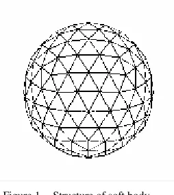
Figure 1. Structure of soft body.

on the surface has six neighboring points where pairs of neighboring points form six triangular faces around point

i

. Gravitational force, spring and damping forces, and internal pressure forces act on point

i

and are used to simulate behavior of the soft body. Calculation of these forces is described next.

A1. Gravitational Force

Gravitational force emanates from the earth, moon, or other massively large objects. The force of gravity experienced by an object on earth is always equal to weight of the object experiencing the gravitational pull. Now, gravitational force experienced by a point on the surface of a soft body is computed by:

g

F

_git

=

m

_i

, (10)

where

F

_git is the gravitational force at time

t

, acting on point

i

of mass

m

_i, and

g

is acceleration due to Earth’s gravity.

A2. Spring and Damping Forces

To simulate elasticity of the soft body, we consider a mass-spring system, in which any two points on the surface of the soft body are connected through springs. A force on one point results in an equal and opposite force on the connected point. A stretched or compressed spring obeys Hooke’s law which states that the force exerted by a coiled spring is linearly proportional to the difference between the stretched or compressed length and rest-length of the spring.

Now, to simulate the surface points on a soft body using this mass-spring system, we consider a point

i

connected to a set of neighboring points. Thus, point

i

experiences spring forces from all

j

that belong to

i

’s connected neighborhood. The cumulative spring force acting on

i

is given by [19]:

∑

∀ ∈

₋

−

−

−

=

_{j ij E}

i j

i j ij i j ij t

i s

x

x

x

x

l

x

x

k

) , ( |

0

|

|

)

(

)

|

(|

F

,

(11)

where

F

_sit is the net internal spring force exerted on point

i

for every point

j

in the neighborhood

E

;

k

_ij is

the spring constant of the spring connecting points

i

and

j

;

x

_i and

x

_jare the positions of points

i

and

j

respectively;

l

_ij0is the rest-length of the spring between points

i

and

j

; and

t

is current time step. Since the spring applies equal and opposite forces to each

connected point pair, it exerts

F

_sit on one point and

t si

F

−

on the connected point.

Along with springs, dampers are typically used in the numerical simulation of soft bodies. A damper connected between two points works against velocity, like viscous drag, to slow down the relative velocity of the two points. For all points

j

, belonging to the connected neighborhood of point

i

on the surface of a soft body, the cumulative damping force,

F

_dit , experienced by point

i

is given by [14]:

∑

∀ ∈

−

=

_{j i j E} ij i j t

di _{|(, )}

k

h

(

v

v

)

F

, (12)

where

F

_di is the damping force,

k

_ijis the damping constant of the damper between points

i

and

j

,

v

_i is the velocity at point

i

,

v

_j is the velocity at point

j

,

t

is current time step, and

h

is time elapsed [14].

A3. Internal Pressure Force

We approximate the internal pressure forces by assuming that there are gas molecules inside the soft body. Since pressure force is the vector sum of the pressure times the area, (1) for point

i

can be modified to consider all surface areas of its neighboring connected points as follows:

∑

∀ ∈

=

_{jk ijk E} ijk t

pi

nRT

V

a

) , , ( |

1

ˆ

n

F

, (13)

where

F

_pit is the net pressure force experienced by point

i

at time

t

,

a

_ijk is surface area of the face connecting point

i

to all point pairs

(

i

,

k

)

in the neighborhood of

i

,

n

ˆ

is a normal vector to the surface where the pressure force is acting,

V

is volume of the body,

n

is the gas mol number,

R

is the ideal gas constant, and

T

is the temperature of the body. We use the Axis Aligned Bounding Box (AABB) [32, 33] to determine volume of the soft body.

B. Combination of All Forces

In this section, we describe how to combine the forces acting at one particular surface point of the soft body. From the previous section, we have all forces, i.e., gravitational force, spring and damping forces and internal pressure forces as follows:

g

F

_git

=

m

_i

∑

∀ ∈

₋

−

−

−

=

_{jij E}

i j i j ij i j ij t i s

x

x

x

x

l

x

x

k

) , ( | 0

|

|

)

(

)

|

(|

F

(11)

∑

∀ ∈

−

=

_{j i j E} t i t j ij t i

d _{|(, )}

k

h

(

v

v

)

F

(12)

∑

∀ ∈

=

_{j i j E} ij t pi

nRT

V

a

) , ( |

1

ˆ

n

F

(13)

Then, the net force

F

_it at point

i

is given by:

t gi t pi t di t si t

i

F

F

F

F

F

=

+

+

+

. (14)

In the next section, we present how to animate soft bodies after calculating the net force at any particular point.

C. Animation with Implicit Integration Method

Our proposed integration method is inspired from [14] and [19] to model 3D soft objects as a 2D grid e.g. cloth. Ref. [19] offers a fast and stable calculation method as compared to [14]. We extend this method to model 3D objects as 3D structures and include an approximation for implicit integration to animate the soft bodies. Rather than computing velocity at each neighboring point, we use an approximation of the forces exerted by neighboring points to generate the velocity at the considered point. Our proposed simplified approximated implicit method bears less computation as compared to the method in [19]. The derived method is described below.

As mentioned earlier, implicit Euler method equations are given by:

i h t i t i h t i

m

h

+ +

₌

_v

₊

_F

v

(8)

h

x

x

_it+h

=

_it

+

v

_it+h

(9)

h t i

+

F

is not easily evaluated at the current value of

,

t i

x

v

_it, and

F

_it, but can be approximated by a first-order derivative as [14, 19]:

h t t h t

_x

x

+ +

_∆

∂

∂

+

=

F

F

F

, (15)

where

F

tis the net force at point

i

, and is given by

F

t

=

[

F

₁t

,

F

₂t

,...,

F

_rt

]

T, where

r

is number of surface points defining the soft body. The difference of

positions,

∆

x

t+h, at times

t

and

t

+

h

, is given by:

t h t h t

x

x

x

=

−

∆

+ +

(16)

It is also written as:

h

x

t+h

=

(

t

+

∆

t+h

)

∆

v

v

_{, (17)}

where

∆

v

t+h is the difference of the velocities at times

t

and

t

+

h

.

To calculate

F

t+h, Desbran et al. [14] use the negated Hessian matrix

x

H

∂

∂

=

F

of the mass-spring system to solve implicit method integration in (15). Substituting (17) in (15), the equation becomes:

h

H

t t h t

h t

)

(

+

+

₌

_F

₊

_v

₊

_∆

_v

F

₍₁₈₎

Then, substituting (18) in (8) and simplifying, we obtain [14]

m

h

h

H

H

m

h

I

)

t h

(

t t

)

(

2

v

F

v

=

+

∆

−

+

(19)

Now, the approximated Hessian matrix is given as [14]:

ij

ij

k

H

=

, if

i

≠

j

; and

∑

≠

−

=

_{j i} ij

ii

k

H

, otherwise,

where

k

is the spring constant.

The calculation in (19) becomes expensive as there is an

n

×

n

matrix

H

involved, where

n

denotes the number of surface points on the soft body. Since

H

_ijis 0 if points

i

and

j

are not linked, the velocity change of point

i

can be updated by considering only the linked points. This approximation leads to [19]:

i t i E j i j j ij i i i ii

m

h

H

m

h

m

H

h

F

v

v

−

∆

=

∆

−

∑

∈ ∀|(, ) 2 2

)

(

)

1

(

(20)

If

k

is constant for all springs, then

H

_iiand

H

_ijcan be approximated as

−

kn

_i and

k

, respectively, to get [19]: i E j i h t j i t i h t i i i i

m

k

h

m

h

m

kn

h

m

∑

_∈

+ +

∆

+

=

∆

+

(, ) 2 2

)

(

F

v

v

.

Simplifying for

∆

v

_it+hand substituting the value

|

|

|

|

_t j t j t j h t j

F

F

v

v

=

∆

∆

+

in (20), we get:

i i E j i t j t j t i h t i

n

kh

m

kh

h

2 ) , (

2

_|

_|

_ˆ

₎

(

+

∆

+

=

∆

+

∑

∈

F

v

F

v

, (21)

We simplify this equation by considering the velocity difference at times

t

and

t

+

h

. In our approximation, the value of

∑

∈

∆

E j i t j t j ) , (

ˆ

|

|

v

F

(22)

is approximated by:

t i t i i

n

|

∆

v

|

F

ˆ

, (23)

where

n

_i is the number of neighbors of point

i

and

F

ˆ

_it

is the normalized force at point

i

, evaluated by

|

|

/

t i t i

F

F

. Equation 22 computes the summation from the number of neighboring surface points that are connected to point

i

, all of which are assumed to be of identical mass and form part of a symmetrical mesh that defines the surface of the soft body. Since this is a mass-spring system, force computed at point

j

is equal and opposite to the force exerted at the connected point

i

. Thus, we have

F

_jt

=

−

F

_it. Now, force is used to compute velocity, as shown in (8). Since we assume the same parameters, i.e. mass, spring and damping constants, for each surface point and each spring, we may

assume

|

∆

v

t_j

|

=

−

|

∆

v

_it

|

without loss of generality. Then, the summation of (22) is approximated by using the number of neighboring points

n

_i multiplied by the magnitude of velocity difference and normalized force at point

i

. Using the approximation of (23) in (21), we get:

(

)

⎟⎟⎠

⎞

⎜⎜⎝

⎛

+

∆

+

=

∆

+ i i t i t i i t i h t i

n

kh

m

n

kh

h

2 2

_ˆ

|

|

v

F

F

v

.

We can simplify the equation as follows:

h t i +

∆

v

i i t i t i i i i t i

n

kh

m

n

kh

n

kh

m

h

2 2 2

ˆ

|

|

+

∆

+

+

=

F

v

F

i t i t i i t i t i i i i t i

n

kh

m

n

kh

n

kh

m

h

2 2 2

|

|

|

|

|

|

F

F

F

v

F

+

∆

+

+

=

(

i i

)

t i t i t i i i i t i

n

kh

m

n

kh

n

kh

m

h

2 2 2

|

|

|

|

+

∆

+

+

=

F

F

v

F

(

i i

)

t i t i t i i t i t i

n

kh

m

v

n

kh

h

2 2

|

|

|

|

|

|

+

∆

+

=

F

F

F

F

(

)

(

i i

)

t i t i i t i t i

n

kh

m

khn

h

2

|

|

|

|

|

|

+

∆

+

=

F

v

F

F

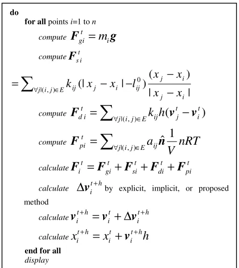
(24)

A summary of simulation steps is shown in Fig. 2. The proposed method takes into account gravitational, spring, damping, and internal pressure forces acting at each point

on the surface of the body. All external and internal forces are calculated and aggregated and then the velocity of point

i

at time

t

+

h

is computed by using either of the explicit, implicit, or proposed implicit methods. The result is passed onto the next step and then a new position is calculated for point

i

. Finally, a display function renders the soft body. This loop repeats until the user terminates the simulation.

IV. METHODS USED FOR COMPARISON

To show that our proposed implicit scheme is stable, we will compare with an explicit integration method. Also, to verify the working of our proposed simplified implicit integration scheme under large spring constants and changing internal pressure forces, we will compare with the implicit Euler integration method of [19]. The simulation will be run under different values of the design parameters: spring constant and gas mole number. Performance of the three methods in terms of frames per second will be analyzed. Also, we will present results of the proposed scheme when multiple soft bodies collide.

Among the three methods, calculation of

∆

v

_it+h

varies. For explicit integration,

∆

v

t_i+h is given by:

i t i h t i

m

h

F

v

=

∆

+ . (25)

If we use the implicit integration by considering the

surrounding points,

∆

v

_it+h is given by [19]:

Figure 2. Steps of simulation

do

for all points i=1 to n compute

F

_git

=

m

_i

g

compute

F

_st_i

∑

∀ ∈

₋

−

−

−

=

_{j ij E}

i j i j ij i j ij

x

x

x

x

l

x

x

k

) , ( | 0

|

|

)

(

)

|

(|

compute

∑

∈ ∀

−

=

_{j i j E} t i t j ij t i

d _{|(, )}

k

h

(

v

v

)

F

compute

∑

∈ ∀

=

_{j ij E} ij t pi

nRT

V

a

) , ( |

1

ˆ

n

F

calculate

F

_it

=

F

_git

+

F

_sit

+

F

_dit

+

F

_pit

calculate

∆

v

t_i+hby explicit, implicit, or proposed method

calculate

v

_it+h

=

v

_it

+

∆

v

_it+h calculate

x

_it+h

=

x

_it

+

v

_it+h

h

end for all

display

i i

E j i

t j t j t

i h t i

n

kh

m

kh

h

2 ) , ( 2

)

ˆ

|

|

(

+

∆

+

=

∆

+

∑

∈

F

v

F

v

(21)

In our proposed implicit integration method by simplified

approximation,

∆

v

_it+h is given by:

(

)

(

i i

)

t i

t i i t

i t i h t i

n

kh

m

khn

h

2

|

|

|

|

|

|

+

∆

+

=

∆

+

F

v

F

F

v

. (24)

Equations (25), (21) and (24) have been used to compare the three methods in different experiments that have been detailed in the next section.

V. EXPERIMENTS

Experiments were conducted for animation and collision detection of soft bodies with 12K faces on a Pentium4 processor running at 3.2 GHz with 512MB NVIDIA GeForce Go 6800 GPU. The experiments provide insight into the performance of explicit, implicit and the proposed simplified implicit method under changing internal pressure forces and large spring constants.

Soft Body Rendering using the Three Methods

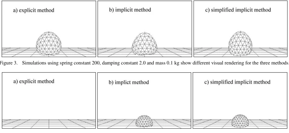
Fig. 3 compares the results between explicit integration, implicit integration [19], and the proposed simplified implicit integration method. The three simulation results show slightly different visual results.

Fig. 4 shows the effect of changing the spring constant of the material. The spring constant is initially set to 500; then, increased to 1000. Fig. 4a shows that the soft body simulation using explicit integration collapses and disappears while the implicit integration method in Fig. 4b and our proposed method in Fig. 4c still generate the soft body animation correctly.

For all simulations, damping constant is 2.0 and mass is 0.1 kg.

Changing Internal Pressure Force in Simplified Implicit Method

This set of experiments was conducted to observe the effect of changing internal pressure forces on the soft body animation generated by our proposed simplified implicit integration method.

Fig. 5 shows results of the simulation when the spring constant is set to 1000 and the gas mol number

n

is switched from 700 to 100 at frame 500. The results show that the soft body simulation generates a realistic deformation when the internal pressure force is changed.

Figure 3. Simulations using spring constant 200, damping constant 2.0 and mass 0.1 kg show different visual rendering for the three methods.

Figure 4. As the spring constant is changed from 500 to 1000, results show that the soft body disintegrates in the explicit integration method while both the implicit methods render the object correctly. Damping constant is set to 2.0 and mass is 0.1 kg.

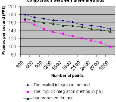
Performance Comparison of the Three Methods

Performance comparison between the explicit integration method, the implicit integration method, and our proposed method is shown in Fig. 6. The comparison is measured in terms of average frames per second (FPS). Spring and damping constants are set at 200 and 2.0, respectively.

The results show that both explicit and our proposed methods perform particularly well even when the number of surface points is increased. The explicit integration method gives better FPS as it requires fewer calculations; however, as mentioned earlier, it becomes unstable when the spring and damping constants are large.

On the other hand, the performance of the implicit integration method [19] drops because the algorithm is computationally expensive. Thus, our proposed method gives a stable, yet efficient simulation.

Collision Interaction using Simplified Implicit Method

Fig. 7 shows collision interaction between many soft body objects using the proposed approximated implicit method. The results show that our proposed method can generate realistic simulation of soft bodies’ collision even when spring constants are large.

VI. APPLICATIONS

The proposed method is efficient and stable and can implement soft body models and props in real-time effectively. Applications include real-time gaming, non-real time graphics, and medical simulations. These applications have soft bodies like balls, bubbles, blob-like creatures, and skin for facial and speech animation. The method can also be used to animate soft objects for non-real time, pre-rendered movie or television special effects. Another application is surgical simulation where the layers of human tissue, such as the layer of muscles in human face, are simulated using mass-spring systems having different stiffness properties [29, 30]. Similarly, the method can be employed in simulating a human lung which expands and contracts with air based on properties and health of the lungs [38].

VII. CONCLUSION AND FUTURE WORK

We have presented a simplified implicit integration method for soft body 3D simulation using a mass-spring system with internal pressure forces.

Our soft body is a mesh of points connected by springs and affected by internal pressure forces that have been modeled after gaseous molecular interactions. An implicit Euler integration method has been used since the explicit approach makes soft body animation unstable under large spring constants with increased stiffness. Specifically, we have extended the 2D implicit integration method of [19] to 3D rendering of objects and propose a simplified approximation for implicit integration to animate our soft bodies. Instead of computing velocity at each neighboring point, we use an approximation of all forces exerted by neighboring points to generate the velocity at a given point. We present comparison with an explicit method and the implicit method of [19] and show that our proposed method produces stable and efficient 3D simulation of soft bodies.

Figure 6. Performance comparison of the three methods: explicit, implicit and proposed implicit.

Future applications include extending the model to simulate soft tissue in medical problems, or to simulate molecular dynamics of different materials. By employing faster collision detection algorithms, the efficiency of the proposed method can be further improved. Additionally, a set of better libraries and bench marks would be designed to compare the algorithm with different models and scenarios.

REFERENCES

[1] J. Teran, S. Blemker, V. Ng Thow Hing, and R. Fedkiw, “Cloth & deformable bodies: Finite volume methods for the simulation of skeletal muscle,” Euro. Symp. on Comp. Anim. (SIGGRAPH Proc.), pp. 68–74, 2003

[2] G. Debunney, M.Desbrunz, M.-P. Caniy, and A. Barrx, “Adaptive simulation of soft bodies in real-time,” Comp. Anim., pp. 133–144, May 2000

[3] D. Nixon, and R. Lobb, “A fluid-based soft-object model,” Comp. Graph. and App., IEEE , Vol. 22 Iss. 4, pp. 68–75, July-Aug. 2002

[4] A. Witkin and D. Baraff , “An Introduction to Physically Based Modeling,” SIGGRAPH Course Notes, 1993. [5] H. B. Callen, Thermodynamics and an Introduction to

Thermostatistics, 2nd edition, John Wiley & Sons, New York, 1985.

[6] D. L. James and D. K. Pai, “Multiresolution green’s function methods for interactive simulation of large-scale elastostatic objects,” ACM Transactions on Graphics (TOG), Vol. 22 Iss. 1, Jan 2003.

[7] S. Cotin, H. Delingette, and N. Ayache , “Real-time elastic deformations of soft tissues for surgery simulation,” Visualization and Computer Graphics, IEEE Transactions on, Vol. 5 Iss. 1 , pp. 62–73, Jan. -Mar 1999.

[8] R. Balaniuk and K. Salisbury, “Dynamic simulation of deformable objects using the Long Elements Method,” Haptic Interfaces for Virtual Environment and Teleoperator Systems, 2002. HAPTICS 2002. Proceedings. 10th Symposium on, pp. 58–65, Mar 2002.

[9] I. F. Costa and R. Balaniuk, “LEM-an approach for real time physically based soft tissue simulation,” Robotics and Automation, 2001. Proceedings 2001 ICRA. IEEE International Conference on, Vol. 3, pp. 2337–2343, 2001. [10] K. Sundaraj, C. Laugier, and I.F.Costa, “An approach to

LEM modeling: construction, collision detection and dynamic simulation,” Intelligent Robots and Systems, 2001. Proceedings. 2001 IEEE/RSJ International Conference on , Vol. 4, 29 Oct. - 3 Nov. 2001

[11] R. Rabaetje, “Real-time simulation of deformable objects for assembly simulations,” Proceedings of the Fourth Australian user interface conference on User interfaces, Vol. 18, 2003

[12] M. Matyka and M. Ollila, “Pressure Model of Soft Body Simulation,” SIGRAD2003, Nov 20-21, 2003

[13] S.F.F Gibson and B. Mirtich, “A Survey of Deformable Modeling in Computer Graphics,” Technical report, Mitsubishi electronic research, 1997

[14] M. Desbrun, P. Schröder, and A. Barr, “Interactive animation of structured deformable objects,” Proc. of Graphics Interface '99, 1999.

[15] M. Kass, “An introduction to continuum dynamics for computer graphics,” In SIGGRAPH Course Notes. ACM SIGGRAPH, 1994.

[16] D. Terzopoulos, J. Platt, and A. Barr, “Elastically deformable models,” Computer Graphics (Proc. of SIGGRAPH '87), pp. 205-214, 1987.

[17] P. Volino, M. Courchesne, and N. Thalmann, “Versatile and efficient techniques for simulating cloth and other deformable objects,” Computer Graphics (Proc. of SIGGRAPH '95), pp. 137-144, 1995.

[18] P. Volino, N. Thalmann, S. Jianhua, and D. Thalmann, “An evolving system for simulating clothes on virtual actors,” IEEE Computer Graphics and Applications, Vol.16, Iss. 5, pp. 42-51, 1996.

[19] Y. Kang, J. Choi, and H. Cho, “Fast and stable animation of cloth with an approximated implicit method,” Proc. Computer Graphics International, 2000.

[20] W. Rechard DeVaul, “Cloth dynamics simulation” master’s thesis, Texas A&M University, Sep 3, 1997. [21] D. Pritchard, “Cloth parameter and motion capture”

master’s thesis, University of Waterloo, 2001.

[22] P. Volino, F. Cordier and N. Magnenat-Thalmann, “From early virtual garment simulation to interactive fashion design”, Computer-Aid Design, Vol 37, Iss. 6, pp. 593-608, May 2005.

[23] A. Fuhrmann, V. Luckas, “Interactive animation of cloth including self collision detection,” Journal of WSCG, Vol 11, Iss 1, pp. 203-208, 2003.

[24] D. Baraff A. Witkin, “Large step of cloth simulation,” International Conference on Computer Graphics and Interactive Techniques, Proceedings of the 25th annual conference on Computer graphics and interactive techniques, pp. 43 – 54, 1998

[25] D.A. Nixon, “A Fluid-Based Soft Object Model” master’s thesis, Univeristy of Auckland, New Zealand, Feb. 1999 [26] M. Meyer, G. Debunne, M. Desbrun, and A. H. Barr,

“Interactive animation of cloth-like object for virtual reality,” The Journal of Visualization and Computer Animation, Vol. 12, Iss. 1, pp. 1-12, May 2001.

[27] M. A. Padilla Castaiieda, F. A. Cosio, “Computer simulation of prostate resection for surgery training,” Proceedings of the 25th Annual International Conference of the IEEE, Vol. 2, pp. 1152-1155, Sep 2003.

[28] X. Provot, “Deformation Constraints in a Mass Spring Model to Describe Rigid Cloth Behavior,” Proceedings of Graphic Interface'95, pp. 147-154, 2005.

[29] K. Waters, “A Physical model of facial tissue and muscle articulation derived from computer tomography data,” Proc. SPIE, Vol. 1808, pp. 574-583, 1992.

[30] E. Keeve, S. Girod, B. Girod, “Craniofacial surgery simulation,” Proceedings of the 4th International Conference on Visualization in Biomedical Computing VBC'96, Hamburg, pp. 541-546, 1996.

[31] M. Teschner, S. Girod, and B. Girod, “Direct computation of nonlinear soft-tissue deformation,” Proc. Vision, Modeling, Visualization VMV'00, pp. 383-390, 2000. [32] G. Van Den Bergen, “Efficient collision detection of

complex deformable models using AABB trees,” Journal of Graphics Tools (USA), Vol. 2, pp. 1-13, 1997.

[33] J. Mesit, E. Hastings, R. Guha, "Muti-level SB Collide: Collision and Self-Collision in Soft Bodies," CGAMES 2006.

[34] O.C. Zienkiewicz and R.L. Taylor. The Finite Element Method. McGraw-Hill, 1991.

[36] M. Kass, An introduction to continuum dynamics for computer graphics. In SIGGRAPH Course Notes. ACM SIGGRAPH, 1994.

[37] S. Nakamura, Initial value problems of ordinary differential equations. In Applied Numerical Methods with Software, pp. 289-350. Prentice-Hall, 1991.

[38] A. P Santhanam, S. N. Pattanaik, J. P. Rolland, and C. Imielinska, “ Physiologically-based Modeling and Visualization of Deformable Lungs”, In Proceedings of the 11th Pacific Conference on Computer Graphics and Applications (PG’03), 2003

Jaurwan Mesit is a Ph.D. student at Department of Electrical Engineering and Computer Science at University of Central Florida. She received her M.Sc. in computer science and B.Sc. in computer science from NIDA (National of Development Administration) and Rajabhat Institute Phetchaburi Thailand in 1992 and 1999, respectively. She is working as a graduated research assistant at University of Central Florida. Her research area is computer graphics in collision detection for flexible objects such as cloths, soft body, and water.

Ratan Guha is a professor at University of Central Florida. He received his B.Sc. degree with honors in Mathematics and M.Sc. degree in Applied Mathematics from University of Calcutta and received the Ph.D. degree in Computer Science from the University of Texas at Austin in 1970. He has authored over 125 papers published in various computer journals, book chapters and conference proceedings. His research has been supported by grants from ARO, NSF, STRICOM, PM-TRADE, NASA, and the State of Florida. He has served as a member of the program committee of several conferences, as the general chair of CSMA’98 and CSMA’2000 and as the guest co-editor of a special issue of the Journal of Simulation Practice and Theory. He is a member of ACM, IEEE, and SCS and served as a member of the Board of Directors of SCS from 2004 to 2006. He is currently serving in the editorial board of two journals: International Journal of Internet Technology and Secured Transactions (IJITST) published by Inderscience Enterprises, and Modelling and Simulation in Engineering published by Hindawi Publishing Corporation.