Haara

COMPARING K NEAREST NEIGHBOURS METHODS AND

LINEAR REGRESSION—IS THERE REASON TO SELECT ONE

OVER THE OTHER?

Arto Haara

, Annika Kangas

1_{Scientist, Joensuu Research Unit, Finnish Forest Research Institute, Finland}

2_{Professor, Department of Forest Sciences, University of Helsinki, Finland}

Abstract. Non-parametric k nearest neighbours (k-nn) techniques are increasingly used in forestry

problems, especially in remote sensing. Parametric regression analysis has the advantage of well-known statistical theory behind it, whereas the statistical properties of k-nn are less studied. In this study, we compared the relative performance of k-nn and linear regression in an experiment. We examined the effect of three different properties of the data and problem: 1) the effect of increasing non-linearity of the modelling task, 2) the effect of the assumptions concerning the population and 3) the effect of balance of the sample data. In order to be able to determine the effect of these three aspects, we used simulated data and simple modelling problems. K-nn and linear regression gave fairly similar results with respect to the average RMSEs. In both cases, balanced modelling dataset gave better results than unbalanced dataset. When the results were examined within diameter classes, the k-nn results were less biased than regression model results, especially with extreme values of diameter. The differences increased with increasing non-linearity of the model and increasing unbalance of the data. The difference between the methods was more obvious when the assumed model form was not exactly correct.

Keywords: Modelling, Regression, Imputation, Balanced Data, K Nearest Neighbour

1

Introduction

Models are needed for almost all forest inventory and planning calculation tasks. For instance, in most cases not all variables of interest are measured for all trees. Typically, some easily measured tree and stand charac-teristicsxare measured on all sample trees (later called tally trees). Characteristics y, whose measurement can be very time-consuming and expensive, are measured only in a smaller sample of trees (later called height sample trees). Models are then used to predict these variablesyfor tally trees as a function of the variablesx

measured for all trees. Besides, the common problem of missing data in forest inventory and planning databases necessitates the use of statistical methods as imputation methods (Eskelson et al.˜2009). Furthermore, a need to forecast the growth and yield in forest management plan-ning is one important reason for the use of statistical methods.

In recent decades, alternatives to traditional regres-sion models, namely non-parametric methods (Fan, 2000), have been increasingly used. The increased use

of non-parametric methods is based on their flexibility compared to corresponding parametric methods (Gib-bons and Chakraborti 1992, Fan 2000). For instance, the non-parametric methods may describe a wider range of non-linear model forms with a large number of possi-ble independent variapossi-bles. They do not require complete knowledge about the model form, and they are based on fewer assumptions. Another justification for the use of many non-parametric methods is their simple applica-tion. However, parametric methods are well known and have a solid statistical theory behind them, for instance, with analytical estimates for model accuracy.

One widely used non-parametric method is the k-nearest neighbour (k-nn) method. In k-nn, the depen-dent variable is predicted as a weighted mean of k near-est observations in a database, where the nearness is defined in terms of similarity with respect to the in-dependent variables of the model. There are a lot of different options available, concerning the selected dis-tance measure, the weighting scheme and the number of neighbours.

With k-nn it is easier to reproduce non-linear

depen-Copyright c2012 Publisher of theMathematical and Computational Forestry & Natural-Resource Sciences

dencies than with parametric methods. On the other hand, obtaining reliable predictions may require a larger dataset with k-nn than with parametric models, as good performance of k-nn requires that allx-values of target units have close neighbours (Magnussen et al.˜2010). In addition, the k-nn method is inevitably biased, as no pre-diction can be larger (smaller) than the weighted mean of largest (smallest) k values of y in the dataset (Mag-nussen et al.˜2010). It means that the extreme values of

y are biased towards the mean. The parametric mod-els are not expected to have this sort of bias within the used data range, but obviously, the predictions can be highly biased in a case of extrapolation. Non-parametric methods retain more of the original (co)variation than parametric models (Moeur and Stage 1995, Kangas and Korhonen 1996, McRoberts et al.˜2002), although the full (co)variation is only preserved with k=1 (Moeur and Stage 1995, McRoberts 2009).

When a random sample is taken from the population, it is often unbalanced. It means that the data is sparse in certain areas, e.g. with a small number of observations having small and/or high values of independent variables (see Vieilledent et al.˜2009). This is adequate for most purposes, but for modelling purposes a balanced sam-ple with an equal number of observations from different parts of data may be more advantageous. Such a sample can be obtained, e.g. with stratified sampling.

There are few studies, in which parametric and non-parametric methods are compared in forest modelling. Vieilledent et al.˜(2009) demonstrated semi-parametric mortality model’s capacity to produce unbiased esti-mates for extreme diameters when compared to para-metric mortality models. Metcalf et al.˜(2009) pre-sented nonparametric Bayesian method for modelling increased mortality of large trees even when data are sparse. The method was compared with the paramet-ric model to place the new estimates within the con-text of previous work on tree mortality. Dobbertin and Biging (1997) used non-parametric classifier CART to model forest tree mortality. In the study CART was also compared with parametric logistic regression. Fehrmann et al.˜(2008) compared linear regression mod-els and k-nearest neighbour approach for estimation of single-tree biomass. Temesgen (2003) examined parame-ter prediction and most similar neighbour approaches to estimate stand tables from aerial information. There are also some studies besides Metcalf et al.˜(2009), in which the influence of sparse data is evaluated (e.g. Vieille-dent et al.˜2009, Maltamo et al.˜2009).

The studied non-parametric and semi-parametric models have been working well compared to the para-metric methods. Each of these studies is a case study, however, and it is not evident whether the differences between the modelling methods are due to the specific

problem or due to the properties of the dataset, or if they are due to the modelling method. The purpose of this study is to analyze the relative performance of k-nn and linear regression in different conditions. We exam-ined the effect of three different properties of the data and problem: 1) the effect of increasing non-linearity of the modelling task, 2) the effect of the assumptions con-cerning the population and 3) the effect of balance of the sample data.

2

Problem Formulation

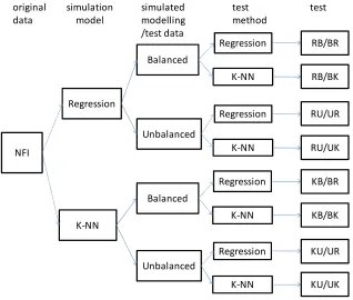
In order to analyse the effect of increasing non-linearity of the modelling task, we compared k-nn method and linear regression in three modelling prob-lems: mean height (stand level data, Norway spruce), height (tree level data, Scots pine) and mortality (tree level data, Scots pine) models. The basic data used for each task was NFI data, to ensure realistic populations (Figure 1). In all modelling cases, we had just one in-dependent variable, the stand mean diameter (DgM) in

stand level models or the tree diameter (_dbh) in tree level models. While more complex models are more com-mon in practise, including several independent variables would have made the experiment more complicated. We also assumed that in a simple experiment the potential differences between the tested methods could be seen more clearly.

In order to analyse the effect of different assumptions concerning the population, we created two artificial pop-ulations for each of the modelling tasks by simulation. This was carried out by simulating the data sets with two different methods, namely a parametric regression model and a k-nn model, with slightly different assumptions (Figure 1). The same methods were later tested in both populations at the modelling stage. This made it possi-ble to examine the effect of the correctness of the used assumptions on the modelling. Finally, we tested the ef-fect of having a balanced or unbalanced sample from the population. The balance here refers to the equal number of observations in different diameter classes. The prob-lems with varying data ranges, as well as the selection of the optimal model shape, were left out from this study. In each of the three modelling cases, we simulated four modelling and corresponding test data sets (Figure 1):

1. Balanced data simulated with parametric regression RB

2. Balanced data simulated with non-parametric k-nn KB

NFI original data

Regression

K-NN simulation

model simulatedmodelling /test data

Balanced

Unbalanced

Balanced

Unbalanced

test test

method

Regression

K-NN

Regression

K-NN Regression

K-NN

Regression

K-NN

RB/BR

RB/BK

RU/UR

RU/UK

KB/BR

KB/BK

KU/UR

KU/UK

Figure 1: The flowchart of the tests carried out in each modelling task, assuming the modelling and test data coming from similarly distributed but independent samples (B/B or U/U).

4. Unbalanced data simulated with non-parametric k-nn KU

The two simulation methods with different assump-tions represent two different populaassump-tions, and the bal-anced and unbalbal-anced set two different samples from each of the populations.

Each modelling and test data set was then used for testing both regression method and k-nn method, producing eight different models and eight different tests: RB/BR, RU/UR, RB/BK, RU/UK, KB/BR, KB/BK,KU/UR,KU/UK (Figure 1). In addition, we made a test where the modelling data were balanced and the test data unbalanced and vice versa, producing additional 8 tests RB/UR, RU/BR, RB/UK, RU/BK, KB/UR, KB/UK,KU/BR,KU/BK. Thus, we used dif-ferent types of samples of each population for modelling and testing. Overall, for each of the three modelling problems there were 16 different tests carried out, but not all the results are shown.

3

Material

The data consisted of observations from the perma-nent sample plots of the Finnish National Forest Inven-tory (NFI) (Valtakunnan... 1986, Tomppo, 2006). All

the Northern NFI plots were excluded from the analysis. The sample plots were measured systematically on field tracts located throughout the country. Each tract included four plots, the centres of which were located 400 m apart (from north to south), the tracts themselves being 16 km apart (from north to south and from east to west). Trees with_dbhlarger than 10 cm were assessed in circular plots of 0.03 hectare and trees with_dbhsmaller than 10 cm in plots of 0.01 hectare. Tree species and_dbh were measured from all trees within plot. Furthermore, each tree within the circle with radius half that of the plot was measured as a height sample tree.

NFI plot data measured in 1995 were used as mod-elling data for mean height (NFI mean height data) and height (NFI height data). NFI plot data measured both in 1985 and 1995 were used as modelling data for mortal-ity (NFI mortalmortal-ity data). The average values for the tree and stratum variables of the plots of the three datasets are presented in Table 1.

4

Methods

4.1 Parametric models Mean height (HgM), tree

Table 1: Summary statistics for tree (height and mortality) and stratum (mean height) characteristics in three NFI data sets.

Data Species n Variable Mean SD Min. Max.

Mean height Spruce 1001 DgM, cm 18.6 8.3 0.7 46.5

Spruce 1001 HgM, m 14.6 6.4 1.6 35.1

Height Pine 6279 _dbh, cm 12.8 7.5 0.3 47.2

Pine 6279 h, m 9.9 5.4 1.4 28.6

Mortality Pine, alive 19673 _dbh, cm 15.5 9.7 0.1 46.0 Pine, dead 654 _dbh, cm 16.1 10.5 0.1 45.0

later also used for modelling in the simulated datasets. In case of mean height, a simple linear regression model with mean diameter (DgM) as an independent variable

was fitted to NFI mean height data

HgM i=a0+a1DgM i+ei (1)

where _a0and _a1 are parameters, _HgM i is the mean

height, _DgM i is the mean diameter andeirandom error

in stand _i. In case of tree height, different parametric regression models with tree_dbhand its modifications as independent variables depending on the model were fit-ted to NFI height data, and the most accurate model was selected. The chosen regression model was

hi=a0+a1dbhi+a2dbh2i+ei (2)

where _a0, _a1 and _a2 are parameters, _hi is the height,

dbhi is the diameter andei random error for treei.

Individual tree mortality was modelled with logistic regression as a parametric model, and was fitted to NFI mortality data. The response variable _p was a binary variable indicating whether tree survives (_p= 1) or dies (_p= 0). _Dbhand some of its modifications were tested as independent variables, and finally_dbhand_dbh2 were chosen as independent variables. The logistic model was formulated as follows:

pi=

1

1 +_e−(a0+a1dbh2_i+a₂dbh2_i) +ei (3) where a_0,a1 and_a2were parameters to be estimated, _pi

is the probability of surviving,_dbhi is the diameter and

ei random error for treei.

4.2 Non-parametric models The k- nearest neigh-bour method (k-nn e.g. H¨ardle 1989, Altman, 1992) was used as a non-parametric method in the three modelling tasks. The estimates of the mean height and height for the target observations were calculated as weighted av-erages of the k nearest observations as

ˆ yj =

k i=1wijyi

k i=1wij

(4)

where _k is a number of nearest neighbours used_{, y}i is

the observed value of dependent variable (mean height HgM, height h or propability p according to the

mod-elling task) of neighbouring tree/stratum _i, ˆ_y is the re-spective prediction for target observation _j and _wij is

the weight of a neighbouring tree/stratum _i for the tar-get tree/stratum_j. The weight was calculated as follows:

wij=

1 1+d_ij

pm

k i=1

1 1+d_ij

pm (5)

where _dij is the similarity distance between i and

j and _pm is the weighting parameter (_i = _j) (e.g. Haara et al.˜1997, Sironen et al.˜2008). It was defined as

dij = L

l=1

cl|xil−xjl| (6)

where _L is the number of independent variables (here one, i. e. dbh or DgM), andc their respective weights.

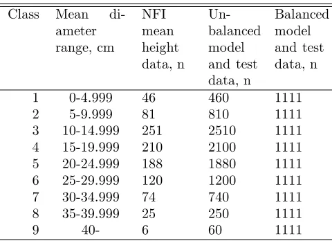
Table 2: Frequencies of observations by mean diameter classes of the NFI mean height data and both simulated balanced and unbalanced datasets.

Class Mean di-ameter range, cm NFI mean height data, n Un-balanced model and test data, n Balanced model and test data, n

1 0-4.999 46 460 1111

2 5-9.999 81 810 1111

3 10-14.999 251 2510 1111

4 15-19.999 210 2100 1111

5 20-24.999 188 1880 1111

6 25-29.999 120 1200 1111

7 30-34.999 74 740 1111

8 35-39.999 25 250 1111

Table 3: Frequencies of trees by diameter classes of the NFI height data and both simulated balanced and unbalanced data.

NFI height data Simulated unbal-anced

Simulated bal-anced

Class Range, cm model test model test model test

1 0-4.999 525 534 525 534 351 347

2 5-9.999 607 623 615 615 342 356

3 10-14.999 985 969 992 962 342 356

4 15-19.999 532 566 546 552 368 330

5 20-24.999 283 244 269 258 338 360

6 25-29.999 117 116 107 126 358 340

7 30-34.999 66 52 63 55 362 336

8 35-39.999 17 29 16 30 346 352

9 40- 7 7 7 7 333 362

Total 3140 3139 3140 3139 3140 3139

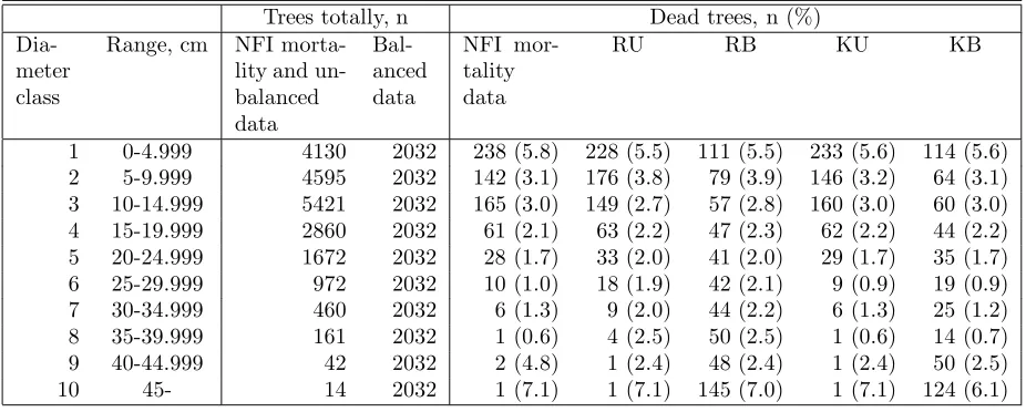
Table 4: Frequencies of trees and dead trees by diameter classes of the NFI mortality data and of the simulated balanced and unbalanced test data. R: regression model, K: k-nn method, U: unbalanced dataset, B: balanced dataset.

Trees totally, n Dead trees, n (%)

Dia-meter class

Range, cm NFI morta-lity and un-balanced data

Bal-anced data

NFI mor-tality data

RU RB KU KB

1 0-4.999 4130 2032 238 (5.8) 228 (5.5) 111 (5.5) 233 (5.6) 114 (5.6) 2 5-9.999 4595 2032 142 (3.1) 176 (3.8) 79 (3.9) 146 (3.2) 64 (3.1) 3 10-14.999 5421 2032 165 (3.0) 149 (2.7) 57 (2.8) 160 (3.0) 60 (3.0) 4 15-19.999 2860 2032 61 (2.1) 63 (2.2) 47 (2.3) 62 (2.2) 44 (2.2) 5 20-24.999 1672 2032 28 (1.7) 33 (2.0) 41 (2.0) 29 (1.7) 35 (1.7) 6 25-29.999 972 2032 10 (1.0) 18 (1.9) 42 (2.1) 9 (0.9) 19 (0.9) 7 30-34.999 460 2032 6 (1.3) 9 (2.0) 44 (2.2) 6 (1.3) 25 (1.2) 8 35-39.999 161 2032 1 (0.6) 4 (2.5) 50 (2.5) 1 (0.6) 14 (0.7) 9 40-44.999 42 2032 2 (4.8) 1 (2.4) 48 (2.4) 1 (2.4) 50 (2.5) 10 45- 14 2032 1 (7.1) 1 (7.1) 145 (7.0) 1 (7.1) 124 (6.1)

The probability of mortality of the target tree was predicted as the proportion of dead trees among the k nearest neighbours. Tree diameter dbh was used as only variable in distance function.

The weighting parameter_pmand the number of near-est neighbours_k were determined using multi-objective optimisation (e.g. Haara 2002). The non-linear pro-gramming algorithm (Hooke and Jeeves 1984) was used to find the combination of decision variables minimis-ing the average absolute difference between the observed and predicted value of each dependent variable (i.e. mean height, tree height, and mortality) using leave-one-out cross-validation. The computer program developed

by Osyczka (1984) was modified and adapted to deal with the _k-nn method. Optimization is needed, when approaches such as canonical correlations (Moeur and Stage 1995) are not used. However, also heuristic search such as genetic algorithm could have been used (Tomppo and Halme 2004). The optimal weighting parameter_pm was 1.445 and the optimal number of nearest neighbours used in the calculations was 30 and 1.445.

of neighbour trees was derived from the number of trees of the diameter class to which the target tree belonged, i.e., in diameter classes, in which the number of trees was smaller fewer neighbours were used.

4.3 Simulated datasets Balanced and unbalanced datasets in regard to the independent variable, dbh or DgM, were generated for each of the three modelling

problems. Observations in the original NFI datasets were grouped to 5 cm dbh/DgMclasses, and the amounts

of observations within each dbh/DgM class were

calcu-lated. In the case of height and mortality datasets, same amount of trees within each dbh class as in NFI height and mortality data were generated randomly for the sim-ulated datasets. In the case of the NFI mean height data the number of observations in each mean diameter class was first multiplied by ten to get the same number of ob-servations than in former two cases (Table 2). In other two cases, the simulated datasets were as large as the original ones (Tables 3 and 4).

In all three datasets most of the observations were middle sized trees. Thus these datasets formed unbal-anced modelling and test datasets. Balunbal-anced modelling and test datasets consisted of same total amount of ob-servations than unbalanced datasets, but the observa-tions were divided approximately evenly between the di-ameter classes.

Then, the values of dependent variables for each three modelling problems were generated using parametric and non-parametric models fitted to the original data. In case of mean height and height models, a normally distributed N(0,_σ2_{) random componentδwas added to} the predictions. The variance of the distribution, _σ 2_, was obtained from the residual variance of the respective models fitted to the original NFI data (Table 3). In the case of parametric regression, we assumed the variance to be heteroscedastic, and simulated the errors using relative standard error (˜_hi = hi(1 +δi)). In the case

of k-nn, we assumed the variance to be homoscedastic, and simulated the random components using a constant (absolute) variance (˜_hi = hi +δi). This was done in

order to produce slightly different populations. For the sake of simplicity, we assumed non-correlated errors. In all k-nn data simulations, the NFI datasets were used as reference datasets.

In case of mortality models, the mortality rate of each generated tree for 10 years period was first predicted with fitted models. The averages of the predicted mor-tality rates of the trees within each class were calculated, and the amount of dead trees was achieved by multi-plying these averages with the amount of trees within diameter class. Dead trees were then selected randomly within each diameter class.

0 5 10 15 20 25 30 35

0 10 20 30 40 50

DGM, cm HG M , m 35 30 25 20 15 10 5 0 35 30 25 20 15 10 5 0 35 30 25 20 15 10 5 0

0______10 ______20 _____30 ______40 ______50

DGM, cm

0______10 ______20 _____30 ______40 ______50

DGM, cm

0______10 ______20 _____30 ______40 ______50

DGM, cm

c)

b)

a)

H

D

H

M

,

m

D

H

M

,

m

D

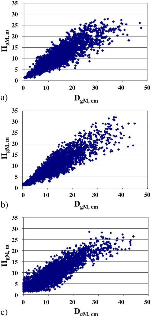
Figure 2: The relationship between mean diameter (DgM) and mean height (HgM) in observed NFI data

(a), and in two simulated unbalanced dataset, generated by utilizing regression model (b) and by utilizing k-nn method (c).

Table 5: Accuracy of the estimates of the mean height models of spruce in different settings and error indexes. R: regression model, K: k-nn method, U: unbalanced dataset, B: balanced data set.

Simulation method Modelling data

Test data

Tested method

RMSE (%)

Bias (%)

Error Index

NFI mean height data U R 16.8 0.00 1.1879

NFI mean height data U K 16.4 0.08 0.1931

R B B R 16.2 -0.84 0.5226

R B B K 17.0 -0.90 0.8473

R U U R 16.8 0.07 0.7625

R U U K 17.7 0.12 0.9170

K B B R 16.0 0.00 1.1292

K B B K 13.6 -0.11 0.0698

K U U R 16.4 0.00 1.2147

K U U K 15.5 1.07 0.2941

R U B R 16.2 -1.2 0.5522

R U B K 16.6 -0.50 0.4951

R B U R 16.8 0.35 0.7298

R B U K 17.5 1.08 0.8272

K U B R 18.2 -4.65 1.1897

K U B K 13.7 0.39 0.1142

K B U R 17.6 3.97 1.1435

K B U K 15.5 0.81 0.1311

as

RM SE=

ni=1 Yi− ∧ Y

i

2

n−1 (7)

bias = 1 n

n

i=1 Yi−

∧ Y_i

, (8)

where Yi denotes the true value of the tree/stratum

characteristics, Yi denotes the predicted value of the

tree/stratum characteristics, and n is the number of trees/strata. The relative RMSEs and biases were ob-tained by dividing estimates of RMSEs and biases by the averages of the true tree/stratum characteristics con-cerned. In addition, we analyzed the accuracy (predic-tion bias and variance) in dbh/DgM classes, and

calcu-lated an error index. The error index was calcucalcu-lated as a mean of absolute differences of each diameter class. In addition, average distances (in the feature space) of the nearest neighbouring tree and 50 nearest trees were calculated within each dataset, i.e. in the NFI data and in the simulated datasets.

In k-nn calculations of the original NFI mean height data, the accuracy was calculated using leave-one-out cross validation because of the smaller amount of obser-vations. In all other cases, k-nn results were calculated using independent modelling and test datasets.

Figure 3: Average mean distances (mm) of the mean diameters of the target trees from the mean diameters of the 50 nearest neighbouring trees by mean diameter classes on unbalanced and balanced model datasets.

5

Results

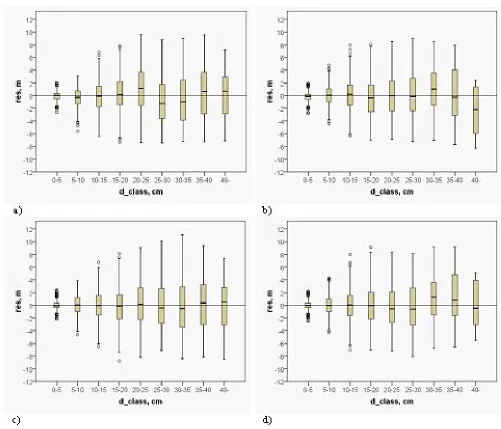
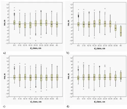
Figure 4: Residuals of mean height in the mean diameter classes for regression model in a) balanced and b) unbalanced data, and for k-nn method in c) balanced and d) unbalanced data. Data were simulated using regression model.

that especially in the case of large trees imitated the true data better than the regression-based dataset: with largest DgM:s the dependency did not seem to be exactly

linear.

The average distances are somewhat different in the NFI data and the simulated datasets. The difference is, however, mostly due to the difference in sizes of these datasets. The differences between balanced and unbal-anced datasets seemed negligible, but when the distances were examined within diameter classes, the distances in the unbalanced datasets were clearly larger than those in balanced data in extreme diameter classes (Fig. 3).

In the original data, the RMSE and error index was

predic-Figure 5: Residuals of mean height in the mean diameter classes for regression model in a) balanced and b) unbalanced data, and for k-nn method in c) balanced and d) unbalanced data. Data were simulated using k-nn method.

tions (Fig. 5), and the error indices of k-nn method were clearly smaller than those with regression model (Table 5). In original data, the differences between the methods were smaller with respect to RMSE than in the simulated data, but with respect to the error index, the differences were as high as in the data simulated with k-nn.

Next we mixed the datasets so that when balanced data were used for modelling, unbalanced data were used for testing and vice versa. It means that the modelling and test data had different distributions. When the data simulation was based on regression, the RMSE of the

k-nn method improved, but that of the regression method remained in the same level (Table 5). When the data simulation was based on k-nn, the RMSE of regression worsened, but that of the k-nn method remained at the same level (Table 5). The average bias level was clearly higher with both methods than in the case of similar test and modelling data.

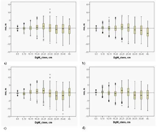
Figure 6: Residuals of the height of the diameter classes of pine for regression model in a) balanced and b) unbalanced data, and for k-nn method in c) balanced and d) unbalanced data. Data were simulated using regression model.

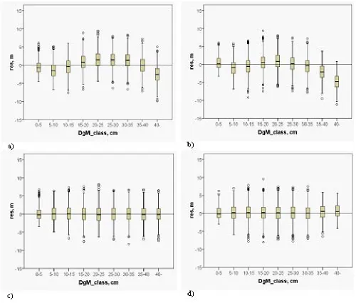
average RMSEs and biases were a little smaller for bal-anced datasets, whereas the differences between the pre-dictions from the regression models and the k-nn method were negligible (Table 6). When regression was the gen-eration method, and the results were examined within diameter classes, the predictions of the k-nn method were a little less biased than regression model predic-tions in both datasets (Fig. 6). The error indices of the nn method were also smaller (Table 6). When the k-nn method was generation method of model and test data, classwise biases, as well as error indices of the k-nn method were clearly smaller than those of regression

(Fig. 7, Table 6).

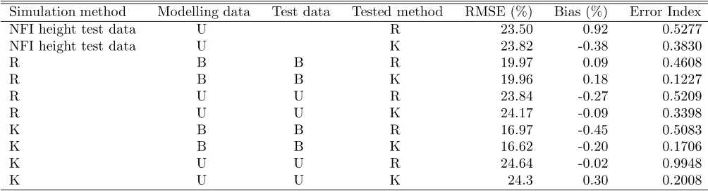
Table 6: Accuracy of the estimates of height models of spruce and error indexes. R: regression model, K: k-nn method, U: unbalanced dataset, B: balanced data set.

Simulation method Modelling data Test data Tested method RMSE (%) Bias (%) Error Index

NFI height test data U R 23.50 0.92 0.5277

NFI height test data U K 23.82 -0.38 0.3830

R B B R 19.97 0.09 0.4608

R B B K 19.96 0.18 0.1227

R U U R 23.84 -0.27 0.5209

R U U K 24.17 -0.09 0.3398

K B B R 16.97 -0.45 0.5083

K B B K 16.62 -0.20 0.1706

K U U R 24.64 -0.02 0.9948

K U U K 24.3 0.30 0.2008

Table 7: Error indexes of mortality models of spruce. R: regression model, K: k-nn method, U: unbalanced dataset, B: balanced data set, LK: locally adjusted k-nn method.

Simulation method Modelling data Test data Tested method Error Index

NFI mortality test data U R 0.007398

NFI mortality test data U K 0.007753

R B B R 0.004532

R B B K 0.000464

R U U R 0.009892

R U U K 0.005252

R U U LK 0.001891

K B B R 0.009947

K B B K 0.000455

K U U R 0.013936

K U U K 0.007179

K U U LK 0.003044

5.3 Mortality models of Scots pine In case of balanced test data generated with regression model, the predictions of both parametric and non-parametric methods were mostly equal (Fig. 8 upper). Only in the predictions of mortality of large trees, the non-parametric model fitted slightly better. The error in-dex was clearly better with k-nn method (Table 7). In unbalanced mortality dataset, in turn, the predictions of the parametric method were highly biased in large diameter classes (Fig. 8 lower). This was also a case for nn method, whereas in case of locally adjusted k-nn method, the predictions were accurate also in large diameter classes. Besides, the error index of locally ad-justed k-nn method was clearly smallest (Table 7).

When the simulated data were generated with k-nn, the differences between methods were more clear. The regression method performed clearly worse than k-nn in balanced (Fig 9 upper), but even more so in unbalanced case (Fig 9 lower). The regression also performed clearly

worse than in the population simulated with regression. When mortality of pine in balanced data was pre-dicted with models, which had been fitted to unbalanced data, the results were similar to the case where both datasets were unbalanced (results not shown). Likewise, in the opposite case, the results were similar to the case where both datasets were balanced. In both cases, the results were determined by the balance of the modelling data.

Figure 7: Residuals of the height of the diameter classes of pine for regression model in a) balanced and b) unbalanced data, and for k-nn method in c) balanced and d) unbalanced data. Data were simulated using k-nn method.

In this study, k-nn method and linear regression were compared in three modelling problems with the relation-ship between the dependent and independent variable varying from linear to highly non-linear. We used sim-ulated datasets, in order to be able to test the influence of assumptions concerning the properties of the popu-lation. The assumptions of interest were that of true model shape and homogeneity of variance. In addition, we examined the effect of balance of the sample data. We used independent test datasets to compare the para-metric and non-parapara-metric methods.

6

Discussion

The datasets used were simulated using either k-nn method or linear regression model as basis, using dbh/DgMas sole independent variable. The populations

Figure 8: Classwise mortality of pine in simulated balanced (upper) and unbalanced (lower) test data and classwise predictions of mortality of logistic model (pred model) and k-nn method (pred knn). Data were simulated using logistic model.

on observations. In this population there is no guaran-tee the used parametric model form is “correct”, even though it was deemed to be the best fitting model. In the former case, we assumed the variance heteroscedas-tic and in the latter case homoscedasheteroscedas-tic. We did not test the compatibility of the generated (unbalanced) test datasets with the true datasets, as with this large a dataset the hypothesis of compatibility is likely to be rejected.

In addition, we assumed all the errors independent. This is a simplification from a true situation. This as-sumption was left for further studies, as the experiment included quite many datasets and assumptions as it is. However, as accounting for the correlations is much less studied in the case of non-parametric methods (see Siro-nen et al.˜2010), it is important to study it in the future. The average RMSEs of the methods were quite simi-lar, and in both cases balanced modelling dataset gave

Figure 9: Classwise mortality of pine in simulated balanced (upper) and unbalanced (lower) test data and classwise predictions of mortality of logistic model (pred model) and k-nn method (pred knn). Simulated data have been generated by k-nn.

better results than unbalanced dataset. It is often as-sumed that k-nn retains the variation original better than regression. In the studied case, with a high number of neighbours, this is not self-evident. However, in un-balanced dataset the k-nn seemed to retain the variation a little better than regression, while in balanced case the situation seemed to be opposite. The variation in both cases seemed more difficult to retain with the extreme values of independent variables.

It can be proved that k-nn results are biased towards the mean with the extreme values of the independent variables (Magnussen et al.˜2010). In the case of regres-sion, this sort of bias should not occur. When the results were examined within diameter classes, the k-nn results were, however, less biased than regression model results with these extreme dbh/DgM classes. The differences

surpris-Figure 10: Standard deviations of a) the observed and predicted heights in balanced data and b) the observed mean heights and predicted mean heights in unbalanced data with respect to diameter classes.

ing that even when the true model form was known (i.e. the fitted model had the same form that was used as a basis for the simulation), and the non-linearity was light or nonexistent, parametric models produced mod-els with increasing bias in the largest diameter classes in an unbalanced data (Fig. 4, 6 and 8). It seems thus that parametric models are not safe from the bias at the extremes, although that bias cannot be analytically de-rived in the same way as for the non-parametric models. In this study, the datasets were generated with two different methods, namely regression and k-nn. In all three cases, regression performed clearly better in dataset generated with regression than with k-nn. Like-wise, k-nn performed better when the data were gen-erated with k-nn rather than with regression. This is not a surprise as such. What is more interesting is that in this case also the differences between regression and k-nn were more pronounced (Fig. 5, 7 and 9).

This is most probably due to the fact that in the first one, the model is smooth and its correct form is

known while in the latter, the model is not necessarily as smooth and the correct form is not exactly known. Thus, it seems that parametric regression is very sensi-tive to the form of the true model, while the k-nn is not. The best performance of linear regression can then only be achieved when the true model form is known.

The variance assumptions did not seem to have any marked effect here. Even when the datasets were mixed so that the modelling dataset was heteroscedastic and the test data were homoscedastic or vice versa, the vari-ance assumption did not seem to have any effect. On the other hand, it is possible that the heteroscedastic dataset has influential observations, i.e. observations that have extreme diameter and a large error, which may affect to the coefficients of the model. This may partly ex-plain the bias in the largest diameter classes. If so, then studying this effect is important in the future. Anyway, it seems that k-nn is safer against such influential ob-servations. The locally adjusted k-nn was only tested with respect to mortality model, but it seems to give the best results in all different cases, and it is thus the most robust of the studied methods.

This result, however, requires that the modelling and test datasets have a similar distribution: if the distribu-tions are different, for instance the ranges of the datasets are not similar, regression model may be more robust. In the studied cases, the differences between the distri-butions were examined by mixing balanced and unbal-anced datasets, i.e. by examining if model estimated with balanced data works well in unbalanced test data and vice versa. In this analysis, regression-based model performed almost as well as in the original cases, pro-vided the true model form was known (Tables 5 and 6). Nonetheless, especially in case of high non-linearity, like mortality with respect to diameter, use of balanced data as a modelling data can produce more accurate estimates in unbalanced test data compared with situa-tion, in which independent unbalanced data are used as a modelling data and balanced data as a test data.

Acknowledgements

The authors wish to thank the anonymous referees for their efforts in improving our text. This work was funded by the Academy of Finland (Decision No. 116313).

References

Altman, N.S. 1992. An introduction to kernel and nearest-neighbor nonparametric regression. Journal of the American Statistical Association 46: 175–185.

Dobbertin, M. and G.S. Biging. 1997. Using the non-parametric classifier CART to model forest tree mor-tality. For. Sci. 44(4): 507–516.

Eskelson, B.N.I., H. Temesgen, V. LeMay, T.M. Barrett, N.L. Crookston, and A.T. Hudak. 2009. The roles of nearest neighbor methods in imputing missing data in forest inventory and monitoring databases. Scand. J. For. Res. 24(3): 235–246.

Fan, J. 2000. Prospects of nonparametric modelling. Journal of American Statistical Association 95: 1296– 1300.

Fehrmann, L., A. Lehtonen, C. Kleinn, and E. Tomppo. 2008. Comparison of linear and mixed-effect regres-sion models and a k-nearest neighbour approach for estimation of single-tree biomass. Can. J. For. Res. 38: 1–9.

Gibbons, J.D. and S. Chakraborti. 1992. Nonparamet-ric statistical inference. Third Edition. Marcel Dekker, Inc. New York, 544 p.

Kasvuennusteiden luotettavuuden selvitt¨aminen knn-menetelm¨all¨a ja monitavoiteoptimoinnilla. Mets¨atieteen aikakauskirja 3/2002: 391–406. (In Finnish)

Haara, A., M. Maltamo, and T. Tokola. 1997. The k-nearest-neighbour method for estimating basal-area diameter distribution. Scand. J. For. Res. 12: 200– 208.

Hamilton, D.A. 1990. Extending the range of applicabil-ity of an individual tree mortalapplicabil-ity model. Can. J. For. Res. 20: 1212–1218.

H¨ardle, W. 1989. Applied nonparametric regression. Cambridge University Press. Cambridge, 323 p.

Hooke, R. and T.A. Jeeves. 1961. ‘Direct search’ solution of numerical and statistical problems. Journal of the ACM 8: 212–229.

Magnussen, S., E. Tomppo, and R.E. McRoberts. 2010. A model-assisted k-nearest neighbour approach to re-move extrapolation bias. Scand. J. For. Res. 25: 174– 184.

Malinen, J. 2003. Locally AdapTable Non-parametric Methods for Estimating Stand Characteristics for Wood Procurement Planning. Silva Fennica 37: 109– 120.

Maltamo, M., E. Næsset, O.M. Bollands˚as, T. Gobakke, and P. Packal´en. 2009. Non-parametric prediction of diameter distributions using airborne laser scanner data. Scand. J. For. Res. 24(6): 541–553.

McRoberts, R.E., M.D. Nelson, and D.G. Wendt. 2002. Stratified estimation of forest area using satellite im-agery, inventory data, and the k-Nearest Neighbors technique. Remote Sens. Environ. 82: 457–468.

McRoberts, R.E. 2009. Diagnostic tools for nearest neighbors techniques when used with satellite im-agery. Remote Sens. Environ. 113: 489–499.

Metcalf, C.J.E., S.M. McMahon, and J.S. Clark. 2009. Overcoming data sparseness and parametric con-straints in modeling of tree mortality: a new nonpara-metric Bayesian model. Can. J. For. Res. 39: 1677– 1687.

Moeur, M. and A.R. Stage. 1995. Most Similar Neighbor. An improved sampling inference procedure for natural resource planning. For. Sci. 41: 337–359.

Osyczka, A. 1984. Multicriterion optimization in engi-neering with Fortran programs. Ellis Horwood, Chich-ester, 178 p.

Sironen, S., A. Kangas, M. Maltamo, and J. Kalliovirta. 2008. Localizing of growth estimates using non-parametric imputation methods. For. Ecol. Manage. 256: 674–684.

Sironen, S., A. Kangas, and M. Maltamo. 2010. Com-parison of different non-parametric growth imputation methods in the presence of dependent observations. Forestry 83: 39–51.

Temesgen, H. 2003. Estimating stand tables from aerial attributes: a comparison of a parametric prediction and most similar neighbour methods. Scand. J. For. Res. 18: 279–288.

Tomppo, E. 2006. Finnish NFI, p. 295–308 in: Kangas. A. and M. Maltamo. (eds.), Forest Inventory. Method-ology and Applications. Managing Forest Ecosystems, vol. 10, Springer (2006).

Vieilledent, G., B. Courbaud, G. Kunstler, J-F. Dhˆote, and J.S. Clark. 2009. Biases in the estimation of

size-dependent mortality models: advantages of a semi-parametric approach. Can. J. For. Res. 39: 1430–1443.