(DOI: 10.24874/jsscm.2018.12.01.09)
An Improved Nodal Ordering for Reducing the Bandwidth in FEM
A. Mohseni1, H. Moslemi1*, M.R. Seddighian1
1 Department of Civil Engineering, Shahed University, Tehran, Iran
e-mail: [email protected] *corresponding author
Abstract
In finite element method, reducing the bandwidth of sparse symmetric matrices plays a key role to have an efficient solution. This problem can be simulated as a vertex numbering problem on a graph, where each edge represents two connected nodes in finite element mesh. In this paper, a new algorithm is proposed for a nodal ordering of the standard and randomly structured graphs to reduce the bandwidth of sparse symmetric matrices. A fast search algorithm for the location of pseudo-peripheral nodes is presented. This algorithm results in a bandwidth smaller than or equal to some existing algorithms such as the Cuthill–Mckee (CM) and the modified Gibbs–Poole– Stockmeyer (MGPS). With this approach, the bandwidth is reduced in more than 50% of instances of benchmark tests compared with the outcomes of the existing algorithms.
Keywords: Bandwidth reduction, finite element method, sparse symmetric matrix, pseudo-peripheral nodes.
1. Introduction
Application of the finite element analysis (FEA) in many problems in structural engineering involves the solution of sparse systems of simultaneous equations with the form (1):
Axb (1)
where ‘A’ is a n×n sparse zeros patterned symmetric matrix, called stiffness matrix, ‘x’ is the
unknown variable vector and ‘b’ is the right-hand side vector. ‘n’ denotes the number of degrees
of freedom.
To improve the accuracy of the solution in FEA many degrees of freedom are usually needed which leads to very high computational and memory cost in the analysis process. But if the nodes are reordered properly, the bandwidth of the sparse matrix will be reduced, and a great deal of the computational effort and memory will be conserved.
For the stiffness sparse symmetric matrix A with entries aij, the ith bandwidth of A is defined
as the difference between the first and last non-zero element of the ith row of the matrix. This parameter is correspondent to the maximum difference in the node numbers within element i. The bandwidth of matrix A is defined as the maximum bandwidth of all rows.
max
i
j a
|
0
ij
The minimizing the bandwidth of the stiffness matrix can be studied by using graph theory and its adjacency matrix. In this paper, a renumbering algorithm is proposed which is based on the determined level structure (Doss and Arathi, 2016). They modified the GPS algorithm introducing a pseudo peripheral node finder algorithm. The main feature of the proposed algorithm in this paper is to achieve a predefined bandwidth by an appropriate ordering of the nodes in each level and forward-backward searching through the nodes. This algorithm also can determine that such preset bandwidth is unreachable mathematically. The proposed algorithm is applied to several different types of standard and random structured graphs and the obtained results are compared with the existing algorithms.
The solution of sparse systems of simultaneous equations forms a considerable part of the computational cost needed in finite element analysis. This computational effort is directly proportional to the square of the bandwidth of stiffness matrix. Thus, a lot of algorithms have been proposed for the reduction of the bandwidth of these sparse matrices. These algorithms can be categorized into two main types: direct and iterative algorithms. In direct algorithms, the nodes are renumbered before the construction of the stiffness matrix. The first extensive study of direct methods for bandwidth reduction was proposed by Cuthill and McKee (1969) by an automatic nodal renumbering scheme is known as the Cuthill-McKee (CM) algorithm. They used a spanning tree to find the shortest route tree of the graph model of the structure. Kaveh (1977) improved the algorithm using special types of the shortest route by the appropriate choice of the starting nodes. King and Levy presented algorithms for minimizing the profile and wavefront of a sparse matrix (King, 1970; Levy, 1971). A reversed CM algorithm (RCM) developed by George (1971) that reversed the numbering in CM algorithm and led to the same bandwidth reduction.
In all of these algorithms, the appropriate selection of the starting node plays a key role in bandwidth reduction. In 1976, one of the most popular algorithms for the bandwidth reduction was proposed called GPS algorithm (Gibbs, Poole and Stockmeyer, 1976). This algorithm is based finding the points of a pseudo-diameter to make maximum depth, for example, a pair of vertices which are at a maximum distance apart. The bandwidth reduction in this algorithm is comparable to the previous ones while being several times faster. Sloan (1986) developed an algorithm to reduce the bandwidth using the points of a pseudo-diameter and relabeled the nodes by introducing the priority of each node to determine a good starting point. To select a proper starting node and a suitable transversal for nodal numbering of graph models of skeletal structures, a new connectivity coordinate system has developed (Kaveh, 1991). He also presented a bandwidth reduction method based on ant colony optimization algorithm (Kaveh, 2011). A heuristic algorithm for the purpose of modification of CM algorithm for the pathological cases has been described byEsposito et al.(1998). Boutora et al. (2007) came up with a strategy to apply a reverse numbering for all the triangular mesh nodes in the permutation vector. An improved GPS algorithm was proposed by introducing width-depth ratio to find the pseudo-peripheral nodes with the distance which is the diameter in a graph (Wang et al., 2009; 2012). An easy bandwidth reduction algorithm was presented on standard L-structured and Z-structured graphs (Doss et al., 2011). A method was developed based on modified GPS algorithm to choose the pseudo peripheral nodes of the standard structured and random graphs (Arathi et al. 2012). They recently improved their method and suggested a new algorithm which leads to better results compared to the modified GPS algorithm (Doss and Arathi, 2016).
unnecessary permutations will be deleted from search algorithm and makes the algorithm very fast. Since the search is accomplished with all of the effective permutations, the numbering for the predefined bandwidth will be found if there would be any solution with GPS level numbering. If no number can be assigned to a node, then the predefined bandwidth will be unreachable.
The outline of the paper is as follows. Section 2 introduces the basic concepts and basic procedures of the new algorithm. Pseudo-code of the algorithm is also given in this section. In section 3, several numerical results demonstrating the robustness and the potentiality of the proposed algorithm are presented and compared with the known algorithms. Finally, some concluding remarks are given in Section 4.
2. Nodal ordering algorithm
An appropriate node renumbering of the standard structured or random graphs based on the modified GPS node finder is presented here to reduce the bandwidth of stiffness matrix efficiently. Firstly a preset aim bandwidth is considered, and in each step, all the numbered nodes are checked not to exceed the aim bandwidth. If no numbers would be available to satisfy this condition, a backward renumbering of previous nodes is carried out. If these backward modifications go to the first node no backward modification is applicable, and the aim bandwidth is unreachable, and a larger aim bandwidth should be reconsidered. To reduce the effort of renumbering process the order of nodes for renumbering is determined by an efficient algorithm based on the connectivity degree of the nodes. Before the renumbering process, the level structures are constructed on the base modified GPS algorithm (Doss and Arathi, 2016).
2.1. Preliminary definitions
Let G( , )V E be a standard or random structured graph in which the elements of ( )V G and ( )
E G are sets of nodes and edges, respectively.
( ) { | }
1, 2, , V G v
i i n
(3)
( ) { | }
1, 2, ,
E G E
j j m
(4)
If v
i and vj are connected together,
v vi, j would be a member of E G( )and in adjacency matrix a 0ij .
The level structure as an essential part of the numbering process is defined as the partitioning of the V G( )into subsets ( )
1
L G , ( ) 2
L G , ... , L G( )
k , in which L G1( )is the root node of the level structure and for i1, L G( )
i is the set of all unassigned nodes which are neighbors to nodes in
( ) 1
L G
i .
2.2. Pseudo peripheral node finder algorithm
An appropriate selection of starting nodes will lead to a proper construction of level structures which have an essential role in the bandwidth reduction of the graph. Hence, in this section, a method for finding pseudo peripheral node based on modified GPS is expressed below (Doss and Arathi, 2016):
1) Select a starting node from the all of the possible nodes of graph G with the minimum degree for searching forward and call it “s”.
2) Suppose that V(G) is partitioned to the all possible levels for searching forward as below:
( ) { ( ), ( ),..., ( )}
,1 , 2 ,
L s l s l s l s
f f f f k (5)
Apply the BFS algorithm for the starting node as the first level ( ( ) { }
,1
l s s
f ). Then the nodes which have the shortest distance (ds,h,min) from the node “s” would be obtained as the second level nodes. This procedure would be continued for the other nodes of the graph by increasing the distance from the starting node “s” until the last level with the maximum distance is found.
( ) | { ( ) | ( ) }
, 2, , , , , min
l s v V G d v d
f h h k s h s h (6)
3) According to the constructed level structure, if the last level consists of a single node, the algorithm stops here and will be continued according to section 2.3. Otherwise, an arbitrary node adjacent to the node with the minimum degree in the last level will be chosen and named “e”.
4) Suppose that V G( ) is partitioned to all possible levels for searching backward as below:
( ) { ( ), ( ),..., ( )}
, , 1 ,1
L e l e l e l e
b b k b k b (7)
Now, the node “e” is selected as the starting node (the first level related to the node “e” i.e.
( ) { } ,
l e e
b k ). Then apply the BFS algorithm again. Similar to the step 2, the nodes which have the shortest distance (de,t,min) from the node “e” would be chosen as the second level. This process would go on for the other nodes of the graph forasmuch the last level with the maximum distance from the beginning node “e” is constructed.
( ) | { ( ) | ( ) }
, 1, ,1 , , , min
l e v V G d v d
b t t k e t e t (8)
5) Let E*be the set of nodes having the same forward and backward level numbers as below:
*
( )
( )
,
,
1,...,
E
v
l
s
l
e
f h
b h
h
k
(9)6) Subtract nodes of E* from the graph G and suppose 1
SG ,
2
SG ,…, SG
Z be partitions of the
7) The final numbering of levels for all of the nodes of the graph is determined according to the following conditions:
The level number of the nodes of E*are evident, since they have the same backward and
forward level number. The nodes which are in the greatest subgraph (GSG) would be numbered with the backward level number to connect to the previous layer, and the other subgraphs are numbered according to the forward level number to balance the number of nodes in each layer which leads to fewer bandwidth.
2.3. The proposed node renumbering algorithm
An important step in the proposed algorithm is the renumbering of nodes in each of the level structures. An appropriate arrangement of the nodes in each level will be lead to a reduced final bandwidth of the graph. Therefore a forward-backward method is proposed to find the proper renumbering in each level to satisfy the preset aim bandwidth. After constructing the levels, an appropriate set of numbers can be assigned to the nodes of each level.
Consider the set { , , , } 1 2
N n n n
k
in which k is the number of levels and ni is the number
of nodes in ith level. For the first level (i=1), the nodes are respectively assigned by numbers from the set {1,2,…,ni} with the priority of minimum connection to the second level. Hence, a
node with the minimum connection is assigned by number 1 as a starting point, and then all other nodes are numbered respectively. If some nodes have the same number of connections to the next level, there will be (ni-1)! states of numbering for each node.
For the second level and above (i ≥ 2), a number from the set
1 1
1, 2,...,
1 1 1
i i i
n n n n
i k k k
k k k
can be assigned to each of the nodes in the ith level. Thus, a
permutation of numbers can be assigned to the all nodes in each level which some of them is irrational and sometimes impossible. However, considering the bandwidth as an objective criterion (βe) according to equation (10), it is significantly possible to reduce the states of
numbering considerably for each of the nodes in the ith level (n '
i ).
min( ') min( ')
1
n n
i i e (10)
where
n
i
is a numbered node in the ith level andn
i
1 is an adjacent numbered node in the(i-1)th level. To minimize the effort of renumbering process, the numbering procedure must be carried out for the nodes with the minimum possible cases of numbering. If the assigned number
for each node did not satisfy the chosen bandwidth, the next number from the set
n
i
would beassigned to the node. This procedure would be continued as far as the last node was numbered. If none of the numbers in the set satisfy the bandwidth, the previous level should be considered again and the next number in the set will be assigned and the procedure will go on forward. If the backward modification reaches to the first level and no number in the first set is remained, the numbering process should be iterated from the start point with a new aim bandwidth (βe+1).
A detailed pseudo-code of the proposed algorithm including modified GPS level structure construction (Doss and Arathi, 2016) and node renumbering algorithm is given below:
PROPOSED ALGORITHM (G, fnn[ ]) ◃ Input: A graph G=G(V, E).
◃ Module 1: To find the source vertex s1. for u ∈ V [G] do
degree[u] = length[Adj(u)]
find u∗∈ v[G] with least degree[u] ◃In case of tie choose an arbitrary vertex s1 ← u∗
BFS(G, s1, ds1[ ]) ◃ Module 2: Call BFS algorithm with source vertex s1 for the input graph G
◃to determine the level structure ◃ Input: A graph G=G(V, E), source vertex s1
◃ Output: The array ds1[u] containing shortest distance values for all vertices u ∈ V [G]
◃ from the source vertices s1. for each vertex u ∈ V [G] - {s1} do ds1[u] ← ∞
π[u] ← N I L ds1[s1] ← 0
π[s1] ← N I L Q ← ∅
ENQUEUE(Q,s1) while Q != ∅
do u ← DE QU EU E(Q) for each v ∈ Adj[u] do if ds1[v] = ∞ then π[v] ← u
ds1[v] ← ds1[π[v]] + 1 ENQUEUE(Q,v)
◃ Module 3: To find the second source node s2 for the backward search. ◃ Construction of set S∗ which has all vertices at the last level.
d∗ ← max{ds1[v] : v ∈ G} S∗ ← {v ∈ V [G]/ds1[v] = d∗}
◃ If S∗ contains one vertex then proceed with the final numbering technique fnn[ ]. If |S∗| = 1◃ i.e. if size of S∗ is single element.
then go to module final node numbering fnn[ ] else
◃ Selection of the second source vertex s2 from which backward BFS is performed ◃ From stemp the vertex with minimum degree in the last level is identified
◃ Through stemp the source s2 of the backward BFS is found.
stemp← MINIMUM DEGREE(S∗)◃ calling Module 1 to find the least degree nodes in S∗
s2 ← Adj[stemp] ◃ The vertex s2 which is adjacent to the least degree node stemp is chosen
◃with ties broken arbitrarily.
◃ Module 4: Perform backward BFS with the source vertex s2. ◃ Here, the initial distance value is taken as d∗
BACKWARD-BFS(G, s2, ds2[ ])
◃ Input: A graph G=G(V,E), source vertex s2
◃ Output: The array ds2[u] containing shortest distance values for all vertices u ∈ V [G]
π[u] ← N I L ds2[s2] ← d∗
π[s2] ← N I L Q ← ∅
ENQUEUE(Q,s2) while Q != ∅
do u ← DE QU EU E(Q) for each v ∈ Adj[u] do if ds2[v] = ∞ then π[v] ← u
ds2[v] ← ds2[π[v]] - 1 ENQUEUE(Q,v)
◃ Module 5: Finding the first largest component with ds1[v] = 2. ◃ Separation of the graph into components.
S^ ={ Collection of all vertices v ∈ G/ds1[v] = ds2[v]} G∗ =G-S^◃ Let G
1, G2, . . . , Gk be the k number of components (subgraphs) after the ◃ removal of S^ arranged in the descending order according to their size. ◃ Computing the first largest component in which a vertex with ds1[v] = 2 appears tag←TRUE
for (i=1;i ≤ k and tag;i++) if(v ∈ Gi and ds1[v] = 2)
i∗ = i ◃ i∗ is the first largest component with a vertex v with ds1[v] = 2. tag ← FALSE
◃ Module 6: Fixing the final level numbering.
◃ The level number for all the vertices in the first largest component which contains a vertex with ds1[v] = 2,
◃ the level number is assigned as ds2[v]. For the remaining components, ds1[v] is assigned for all vertices.
for v ∈ V [G]
if v ∈ Gi∗ then l[v]=ds2[v] else
l[v]=ds1[v]
Module 7: Fixing the final node numbering
n = |number of levels| do I = 1 to size(n);
a = |the node that has minimum connection to back levels|; b = |the node that has maximum connection to forward levels|; C = |find possible numbers in level (I) |;
do i = 1 to size(C) A = minimum(C) B = maximum(C)
Creating permutations between A & B Checking aim bandwidth of graph if bandwidth is satisfied
Go to next level; else
Finding the best numbering of graph vertices or graph bandwidth optimization is a NP-Complete problem that cannot be solved in polynomial time on a deterministic Turing machine. After layering procedure, the set of numbers which can use in each layer is clear. Hence, the algorithm can search solutions very quickly. But when the number of vertices in each layer increases, finding the best numbering in each layer turns into a NP-Complete problem. To prevent this shortcoming the proposed algorithm considers a desirable bandwidth and starts from the node with a priority of minimum connection to the next level to satisfy the predefined bandwidth. If the existing bandwidth exceeds desirable bandwidth, then the numbering in layer will change quickly. By this trick and using “for in for” programming for each layer the problem can be solve with an acceptable cost.
3. Numerical examples
To illustrate the capability of the proposed renumbering algorithm, two finite element models are considered in detail. Some other benchmark examples are investigated and the results of reduction bandwidth are summarized in tables 3 and 4. In the finite element analysis, the three-noded triangular elements are used in both examples and their equivalent graphs are constructed. To investigate the effect of proposed renumbering technique, the evaluated reduced bandwidth is compared with the known algorithms such as such as the Cuthill–McKee (CM), the GPS and modified GPS.
3.1. A rectangular plate under tension
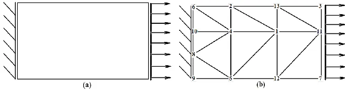
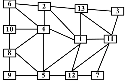
The first example is of a rectangular plate with a finite crack subjected to uniform tension loading. The geometry of the problem and finite element mesh with an arbitrary initial numbering are shown in Fig. 1. The equivalent structured graph is constructed with 13 vertices and initial bandwidth equal to 12 as shown in Fig. 2. The proposed algorithm is described for this graph in detail in two distinctive parts as follows:
Fig. 1. Rectangular plate under tension: a) geometry, b) finite element mesh.
The pseudo peripheral node finder algorithm:
1- From Fig. 2, the node 3 is chosen as the starting node “s” among all possible nodes
with the minimum degree including {3,7,9}.
2- A forward BFS algorithm for the starting node 3 as the first level is applied. This leads to a level structured graph with 5 levels as shown in Fig. 3 (first numbers).
3- In the last level (5th level) consisting of nodes {8,9}, the node 8 as the node adjacent to the node 9 with minimum degree is chosen as the starting node “e” for backward
4- A backward BFS algorithm for the starting node 8 is applied as shown in Fig. 3 (second numbers).
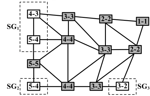
5- The set E* including nodes {3,11,13,12,1,2,5,4,8} with the same forward and
backward level numbers is partitioned (Fig. 4).
6- Subgraphs SG1, SG2 and SG3 are partitioned as illustrated in Fig. 4. Then the
subgraph SG1 as the greatest subgraph (GSG) is numbered with the backward level
number and the subgraphs SG2and SG3 are numbered according to the forward level
number, and final numbering of nodes is obtained as shown in Fig. 5.
Fig. 2. Structured graph of rectangular plate with 13 vertices.
Fig. 4. Subgraphs E*, SG1, SG2 and SG3 of Graph G.
The proposed renumbering algorithm:
1- As shown in Fig. 5, the nodes in each level are respectively assigned by the sets of numbers including {1},{2,3},{4,5,6,7,8},{9,10,11} and {12,13}.
2- For the first level, no.1 from {1} is assigned because it is the lonely single node in this level.
3- For the second level, it is assumed that the aim bandwidth is 2 (βe=2). Due to the
same states of numbering for the nodes 13 and 11, each number from the set {2,3} can be assigned to the nodes arbitrarily.
4- As shown in Fig. 6, by assuming no.2 for the node 13 and no.3 for the node 11 in the 2nd level and βe=2, the set {4,5,6,7,8} would be the possible states of numbering
for the existing nodes in the third level. By allocating no.4, no.5 and no.6 to the nodes 7, 12 and 1, the corresponding bandwidth would be 3. Thus, the numbering procedure is returned to the previous level and the order of node 2,3 are reversed. But the obtained bandwidth would be 3 once more. Hence, the aim bandwidth of 2 is impossible for this graph and βe must be increased to 3. By repeating this
procedure, it can be found that βe=3 was still not satisfied because three nodes are
connected to node 2 and the numbering process must be iterated for all the levels based on βe=4. At last, as depicted in Fig. 7, in the third level set of {4,5,6} is
Fig. 5. Final numbering of levels and sets of assigned numbers for each level.
Fig. 6. Bandwidth changes by renumbering the nodes in each level.
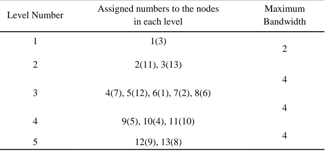
The assigned numbers to the nodes in each level and maximum obtained bandwidth for each level are presented in Table 1.
Level Number Assigned numbers to the nodes in each level
Maximum Bandwidth
1 1(3)
2
2 2(11), 3(13)
4
3 4(7), 5(12), 6(1), 7(2), 8(6)
4
4 9(5), 10(4), 11(10)
4
5 12(9), 13(8)
Table 1. Maximum obtained bandwidth for each level.
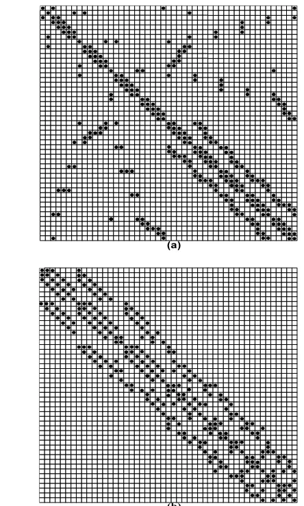
Fig. 8. Rectangular plate: Bandwidth of the interconnectivity matrix, a) Initial bandwidth, b) Reduced bandwidth.
Fig. 8 shows the performance of bandwidth reduction in the interconnectivity matrix based on renumbering the nodes of the graph. The original matrix bandwidth with initial numbering and the resultant matrix bandwidth after applying the proposed renumbering algorithm are shown in Fig. 8.a and Fig. 8.b respectively. It demonstrates the improvement in the bandwidth reduction process.
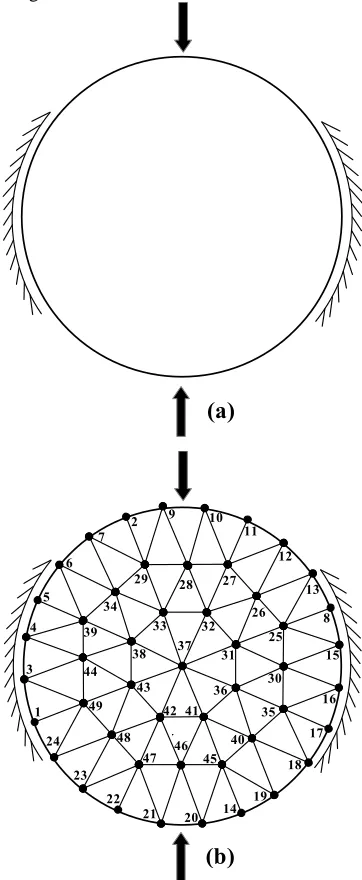
3.2. A circular plate under concentrated loads
The pseudo peripheral node finder algorithm:
As shown in Fig. 10, from all minimum possible degree nodes consisting of {1,2,5,8,11,14,17,22}, the node 1 is selected as the starting node “s”. By applying a forward BFS
algorithm for the node 1 as the first level, a level structured graph with 7 levels is obtained. Then the node 16 adjacent to a node with minimum degree at last level (7th level) is chosen from {2,9,10,11,12,13,8,15,16,17,18,19,14} to be the starting node “e” for backward search. The set E* is constructed including nodes {1,49,43,37,31,36,35,30,16}. The final numbering of levels is accomplished as shown in Fig. 11.
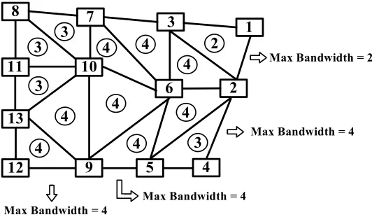
Fig. 10. Equivalent structured graph of circular plate with 49 vertices.
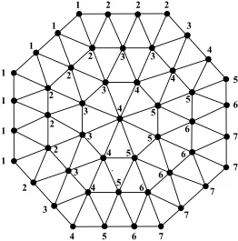
Fig. 12. Final renumbering of the nodes with maximum bandwidth of 9.
The proposed renumbering algorithm:
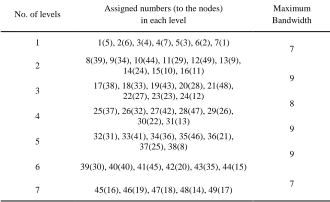
The implemented renumbering algorithm in this example is similar to the previous one. The smallest bandwidth of this graph with well-known algorithms was 10 and thus, aim bandwidth is taken 9 to investigate the improvement ability of the proposed algorithm. The node 5 with the minimum connection to the second level is selected as the starting node is selected and the algorithm proceeded level by level. In each level, retaining aim bandwidth is checked and some forward-backward modification is also carried out to final renumbering is achieved as shown in Fig. 12. The maximum bandwidth between levels is attained according to the Table 2.
No. of levels Assigned numbers (to the nodes) in each level
Maximum Bandwidth
1 1(5), 2(6), 3(4), 4(7), 5(3), 6(2), 7(1)
7
2 8(39), 9(34), 10(44), 11(29), 12(49), 13(9), 14(24), 15(10), 16(11)
9 3 17(38), 18(33), 19(43), 20(28), 21(48),
22(27), 23(23), 24(12)
8 4 25(37), 26(32), 27(42), 28(47), 29(26),
30(22), 31(13)
9 5 32(31), 33(41), 34(36), 35(46), 36(21),
37(25), 38(8)
9 6 39(30), 40(40), 41(45), 42(20), 43(35), 44(15)
7 7 45(16), 46(19), 47(18), 48(14), 49(17)
Fig. 13. Circular plate: Bandwidth of the interconnectivity matrix, a) Initial bandwidth, b) Reduced bandwidth.
NO. No. of
nodes No. of edges
Original bandwidth
Reduced bandwidth
CM GPS Modified
GPS
Proposed algorithm
1 13 25 12 5 5 4 4
2 24 68 48 7 5 5 5
3 34 96 20 9 8 8 8
4 49 119 48 15 12 10 9
Table 3. A comparison of reduced bandwidth in proposed algorithm with CM, GPS and modified GPS on some standard graphs.
NO. No. of
nodes Structures
Original bandwidth
Reduced bandwidth
CM GPS Modified GPS Proposed algorithm
1 21 L-Structured
with 7-point 6 7 7 7 5
2 33 L-Structured
with 7-point 8 7 7 6 5
3 21 L-Structured
with 9-point 6 7 7 6 6
4 33 L-Structured
with 9-point 8 7 7 6 6
Table 4. A comparison of reduced bandwidth in proposed algorithm with CM, GPS and modified GPS on some L-structured graphs.
(a) (b)
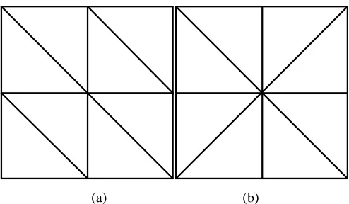
Fig. 14. Formation of a) a 7-point L-structured graph, b) a 9-point L-structured graph.
4. Conclusion
improve the bandwidth reduction process. The technique was associated with the modified GPS algorithm to provide an efficient level structure construction. In this algorithm, the priority of nodes was modified to reduce the effort of renumbering process based on the connectivity degree of the nodes. The aim bandwidth can be chosen, so that overcomes the bandwidth obtained by other well-known algorithms. A forward-backward modification is presented to control the certainty of the aim bandwidth in different levels. This algorithm also can determine that such predefined aim bandwidth is reachable or not with the constructed level structure. Several numerical examples were modeled with arbitrary graphs. It was shown how the proposed renumbering algorithm could reduce the value of bandwidth of stiffness matrix considerably in L-structured graphs.
References
Arathi P, Doss LJT and Kanakadurga K (2012). A constructive bandwidth reduction algorithm.
International Journal of Operational Research, 15(3): 308-320.
Boutora Y, Takorabet N, Ibtiouen R and Mezani S (2007). A new method for minimizing the bandwidth and profile of square matrices for triangular finite elements mesh. IEEE Transactions on Magnetics, 43(4): 1513-1516.
Cuthill E, McKee J (1969). Reducing the bandwidth of sparse symmetric matrices, In
Proceedings 24th, National Conference ACM. pp. 157-172.
Doss LJT, Arathi P (2011). A bandwidth reduction algorithm for L-shaped and Z-shaped grid structured graphs. Operations Research Letters, 39(6): 441-446.
Doss LJT, Arathi P (2016). A constructive bandwidth reduction algorithm-A variant of GPS algorithm. AKCE International Journal of Graphs and Combinatorics, 13(3): 241-254. Esposito A, Catalano MF, Malucelli F and Tarricone L (1998). A new matrix bandwidth reduction
algorithm. Operations Research Letters, 23(3-5): 99-107.
George A (1971). Computer implementation of the finite element method. STAN CS-71-208, Computer Science Department, Stanford University, Stanford, California.
Gibbs NE, Poole WG and Stockmeyer PK (1976) An algorithm for reducing the bandwidth and profile of a sparse matrix. SIAM Journal on NumericalAnalysis, 13(2): 236-250.
Kaveh A (1977). Topological study for the bandwidth reduction of structural matrices. J. Sci. Tech.: 27-36.
Kaveh A (1991). Connectivity coordinate system for node and element ordering. Comput & Structures, 41(6): 1217–1223.
Kaveh A, Sharafi P (2009). Nodal ordering for bandwidth reduction using ant system algorithm.
Int. J. Comput. Aided Eng. Softw, 26(3): 313–323.
King IP (1970). An automatic reordering scheme for simultaneous equations derived from network systems. International Journal for Numerical Methods in Engineering 2(4): 523-533.
Levy R (1971). Resequencing of the structural stiffness matrix to improve computational efficiency. Jet Propulsion Laboratory Quart. Tech. Review, pp. 61-70.
Sloan SW (1986). An Algorithm for Profile and Wavefront Reduction of Sparse Matrices.
International Journal for Numerical Methods in Engineering, 23(2): 239-251.
Wang Q, Guo YC and Shi XW (2009). An improved algorithm for matrix bandwidth and profile reduction in finite element analysis. Progr. Electromagn. Res. Lett. 9(1): 29-38.