Modeling of Machining Operation for CNC Turning AISI1040 Using Response Surface Methodology

(1)

Modeling of Machining Operation for CNC Turning

AISI1040 Using Response Surface Methodology

N.E. EDWIN PAUL

1

, P. MARIMUTHU

2

, K. CHANDRASEKARAN

3

and P. MURUGESAN

4

1 _{Research Scholar, Department of Mechanical Engineering, Bharath University, Chennai -600 073.}

Email ID:[email protected](Corresponding author).

2

Principal and Professor, Department of Mechanical Engineering, Syed Ammal Engineering College, Ramanathapuram-623502, Tamilnadu, India. Email ID: [email protected].

3 _{Assistant Professor, Department of Mechanical Engineering, Nadar Saraswathi College of Engineering and Technology, Theni,}

Tamilnadu, India. Email ID: [email protected].

4

Principal and Professor, Department of Mechanical Engineering, Odaiyappa College of Engineering & Technology, Theni-625531, Email ID:[email protected]

Abstract-- AISI1040 parts that carry critical loads in everything from automotive drive trains and jet engines to industrial bearings are produced by a series of processes, including time consuming and costly grinding and polishing operations. The main objective of machining is to produce a product of required shape and dimension with specific quality and surface finish. But cutting parameters are affecting the quality of process such as surface finish and material removal rate. The modern industry requires better way of machining that will not affect the quality of the product. Response surface design (RSD) is effective tool for modeling and it is solved by second order polynomial equation. So in this investigation, RSD is used for modeling and prediction of machining parameters on AISI1040 using TiCN/TiN and TiAlN coated tool under dry condition.

Index Term--

AISI1040; CNC turning; TiCN/TiN; TiAlN; Response surface design

I INTRODUCTION

Steel is an alloy of iron with definite percentage of carbon ranging from 0.15-1.5%. Steel with low carbon content has the same properties as iron i.e. soft but easily formed [1]. As carbon content rises, the metal becomes harder and stronger but less ductile. Medium carbon steels are used for fabrication. In addition, machined parts such as bolts, turbine casing and concrete reinforcing bars are made of this class of carbon steel. Gears, wire rods, seamless tubing, hot-rolled/cold finished bars and forging products are also some objects constructed from medium carbon steel. The reason for its importance is that it is a tough, ductile and cheap material with reasonable casting, working and machining properties, and also amenable to simple heat treatments to produce a wide range of properties [2, 3]. To have good surface finish, one has to machine a component in multiple cuts. The machining concept of multiple cuts machining increases the processing time, production cost and high setup time. Hence, hard turning operation where components are machined with single cut operation came into existence to focus on reduction in processing time, production cost and setup time with high surface finish [4]. Surface roughness is one of the most important customer requirements and is an indicator of quality in metal cutting machining process. Surface Roughness is not just a single property, because it plays a major role in focusing attention on the product appearance, functionality and assembly [5]

Turning is one of the most common methods for cutting and especially for the finishing of components. The goal of the modern industries is to manufacture low cost, high quality products in short time. In turning, to achieve high cutting performance, selection of optimum parameters is very essential. It has long been recognized that cutting conditions such as feed rate, cutting speed and depth of cut in machining operation should be selected to optimize the economics of machining operations as assessed by productivity, total manufacturing cost per component or some other suitable criteria [6,7]. However, it is very difficult to control all the parameters at a time that affect the surface roughness and material removal rate for a particular manufacturing process. In a turning operation, it is a vital task to select the cutting parameters properly to achieve the high quality performance. Generally, the desired cutting parameters are selected based on experience or use by the hand book. But a better result may be achieved by modeling and optimization of cutting parameters. Several mathematical models based on statistical regression or neural network techniques have been constructed to establish the relationship between the cutting performance and cutting parameters [8,9]. Various compositions of cutting tools were used by past researchers for turning. But response surface regression on AISI1040 in CNC turning TiCN/TiN and TiAlN coated cutting tool were not carried out by them. So, in this investigation, RSD is used for prediction of Reponses such as SR and MRR in turning AISI1040 with different coated cutting toolusing response surface design.

(2)

two design types is that the BBD has no points at the vertices of the cube defined by the ranges of the factors. This is sometimes useful when it is desirable to avoid these points due to engineering considerations. The price of this characteristic is the higher uncertainty of prediction near the vertices compared to the central composite design [10, 11].

II EXPERIMENTAL DETAILS

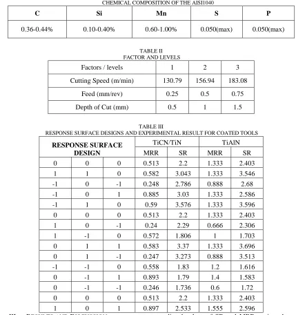
The work piece materials selected for all the trials are AISI1040. The chemical composition of the work piece material is given in Table 1. Experiments were conducted on

CNC Fanuc lathe using AISI1040 steel rods of 22.8 mm diameter and 30 mm of machined length. Three operating factors such as depth of cut, feed and cutting speed have been selected for parametric optimization and each parameter has three levels are given in Table 2. The SR was measured using Mitutoyo Surf Tester 211 with a cut off length of 0.25 mm. In this investigation the TNMG 120408 coated with TiCN/TiN and TiAlN coated tools are used as the insert for turning operation.

TABLE I

CHEMICAL COMPOSITION OF THE AISI1040

C Si Mn S P

0.36-0.44% 0.10-0.40% 0.60-1.00% 0.050(max) 0.050(max)

TABLE II FACTOR AND LEVELS

Factors / levels 1 2 3

Cutting Speed (m/min) 130.79 156.94 183.08

Feed (mm/rev) 0.25 0.5 0.75

Depth of Cut (mm) 0.5 1 1.5

TABLE III

RESPONSE SURFACE DESIGNS AND EXPERIMENTAL RESULT FOR COATED TOOLS

RESPONSE SURFACE DESIGN

TiCN/TiN TiAlN

MRR SR MRR SR

0 0 0 0.513 2.2 1.333 2.403

1 1 0 0.582 3.043 1.333 3.546

-1 0 -1 0.248 2.786 0.888 2.68

-1 0 1 0.885 3.03 1.333 2.586

-1 1 0 0.59 3.576 1.333 3.596

0 0 0 0.513 2.2 1.333 2.403

1 0 -1 0.24 2.29 0.666 2.306

1 -1 0 0.572 1.806 1 1.703

0 1 1 0.583 3.37 1.333 3.696

0 1 -1 0.247 3.273 0.888 3.513

-1 -1 0 0.558 1.83 1.2 1.616

0 -1 1 0.893 1.79 1.4 1.583

0 -1 -1 0.246 1.736 0.6 1.72

0 0 0 0.513 2.2 1.333 2.403

1 0 1 0.897 2.533 1.555 2.596

III RESULTS AND DISCUSSION

Fifteen Reponses are observed for modeling using the second order polynomial equation. From the experimental data, quadratic regression models are obtained. Table 3 shows the RSD of experiments with cutting speed, feed and depth of cut for TiCN/TiN and TiAlN. Table 4 shows the RSD of

(3)

TABLE IV

PREDICTED VALUES FOR COATED TOOLS

RESPONSE SURFACE DESIGN

TiCN/TiN TiAlN

MRR SR MRR SR

0 0 0 0.513000 2.20000 1.33300 2.40300

1 1 0 0.537875 3.00525 1.32738 3.50625

-1 0 -1 0.286625 2.77350 0.92413 2.64863

-1 0 1 0.845875 2.93350 1.34688 2.51713

-1 1 0 0.546375 3.64725 1.27737 3.65650

0 0 0 0.513000 2.20000 1.33300 2.40300

1 0 -1 0.279125 2.38650 0.65213 2.37487

1 -1 0 0.615625 1.73475 1.05563 1.64250

0 1 1 0.665750 3.39525 1.37475 3.70438

0 1 -1 0.252000 3.21425 0.90750 3.48388

-1 -1 0 0.602125 1.86775 1.20563 1.65575

0 -1 1 0.888000 1.84875 1.38050 1.61213

0 -1 -1 0.163250 1.71075 0.55825 1.71163

0 0 0 0.513000 2.20000 1.33300 2.40300

1 0 1 0.858375 2.54550 1.51888 2.62738

Table V and Table VI gives an insight into the linear, quadratic and interaction effects of the parameters for TICN/TIN. These analyses are done by Fisher’s ‘F’ and Student ‘T’ tests. This test is used to determine the significance of the regression coefficients of the parameters. The P value is used as a tool to check the significance of each factor and interaction between factors. The larger magnitude of T and smaller the values of P are more significant in corresponding coefficient term. It is found that the variable with the largest effect on MRR is the linear effect of depth of cut having a T value of 10.857 followed by interaction effect of feed and depth of cut with T value of 2.097. The linear effect of cutting speed is found to be insignificant with T value of 0.048.

The results in Table 6 shows the RSD of SR and indicate that linear effect of feed having a T value of 24.077 followed by linear effect of cutting speed with T value of 6.118. The interaction effect of cutting speed and depth of cut is found to be insignificant with T value of 0.006. The models are then checked using a numerical method employing the coefficient of determination (R2), adjusted R2 (R2adj). R2 indicates how much of the observed variability in the data is accounted for by the model, while R2adj modifies R2by taking into account the number of predictors in the model. The response surface models are developed in this study with values of R2 say 96.2% and 99.3% for SR and MRR respectively. Furthermore, an R2adj close to the R2 values insure a satisfactory adjustment of the quadratic models to the experimental data.

TABLE V

RESPONSE SURFACE REGRESSIONS: MRR VERSUS A, B, C FOR TICN/TIN

Term Coef SE Coef T P

Constant 0.513000 0.04281 11.983 0.000

A 0.001250 0.02622 0.048 0.964

B -0.033375 0.02622 1.273 0.259

C 0.284625 0.02622 10.857 0.000

A*A 0.068875 0.03859 1.785 0.134

B*B -0.006375 0.03859 0.165 0.875

C*C -0.014375 0.03859 0.373 0.725

A*B -0.005500 0.03707 0.148 0.888

A*C 0.005000 0.03707 0.135 0.898

B*C -0.077750 0.03707 2.097 0.090

S = 0.07415 R-Sq = 96.2% R-Sq(adj) = 89.4%

TABLE VI

RESPONSE SURFACE REGRESSIONS: SR VERSUS A, B, C FOR TICN/TIN

Constant 2.20000 0.05172 42.540 0.000

A -0.19375 0.03167 6.118 0.002

B 0.76250 0.03167 24.077 0.000

C 0.07975 0.03167 2.518 0.053

A*A 0.24062 0.04662 5.162 0.004

B*B 0.12313 0.04662 2.641 0.046

C*C 0.21912 0.04662 4.701 0.005

A*B -0.12725 0.04479 2.841 0.036

A*C -0.00025 0.04479 0.006 0.996

B*C 0.01075 0.04479 0.240 0.820

(4)

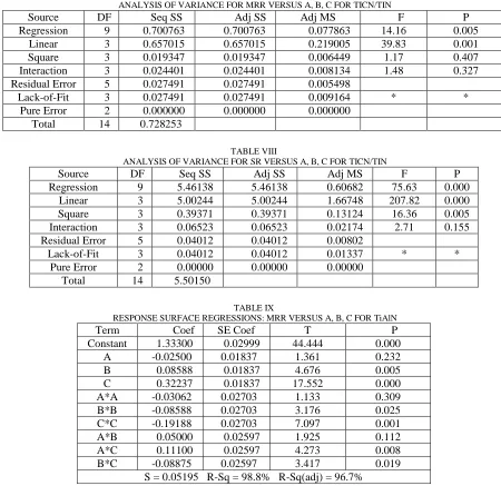
The ANOVA on these models for MRR and SR of TICN/TiN is shown in Table VII and Table VIII. It demonstrates that the models are highly significant, as evident from the very low probability of P values in the regression 0.005 and 0.000 for MRR and SR. The results of the lack of fit test for the models

are shown in Table VII and Table VIII. The lack of fit test describes the variation in the data around the fitted model. If the model does not fit the data well, the lack of fit is not significant.

TABLE VII

ANALYSIS OF VARIANCE FOR MRR VERSUS A, B, C FOR TICN/TIN

Source DF Seq SS Adj SS Adj MS F P

Regression 9 0.700763 0.700763 0.077863 14.16 0.005

Linear 3 0.657015 0.657015 0.219005 39.83 0.001

Square 3 0.019347 0.019347 0.006449 1.17 0.407

Interaction 3 0.024401 0.024401 0.008134 1.48 0.327

Residual Error 5 0.027491 0.027491 0.005498

Lack-of-Fit 3 0.027491 0.027491 0.009164 * *

Pure Error 2 0.000000 0.000000 0.000000

Total 14 0.728253

TABLE VIII

ANALYSIS OF VARIANCE FOR SR VERSUS A, B, C FOR TICN/TIN

Regression 9 5.46138 5.46138 0.60682 75.63 0.000

Linear 3 5.00244 5.00244 1.66748 207.82 0.000

Square 3 0.39371 0.39371 0.13124 16.36 0.005

Interaction 3 0.06523 0.06523 0.02174 2.71 0.155

Residual Error 5 0.04012 0.04012 0.00802

Lack-of-Fit 3 0.04012 0.04012 0.01337 * *

Pure Error 2 0.00000 0.00000 0.00000

Total 14 5.50150

TABLE IX

RESPONSE SURFACE REGRESSIONS: MRR VERSUS A, B, C FOR TiAlN

Constant 1.33300 0.02999 44.444 0.000

A -0.02500 0.01837 1.361 0.232

B 0.08588 0.01837 4.676 0.005

C 0.32237 0.01837 17.552 0.000

A*A -0.03062 0.02703 1.133 0.309

B*B -0.08588 0.02703 3.176 0.025

C*C -0.19188 0.02703 7.097 0.001

A*B 0.05000 0.02597 1.925 0.112

A*C 0.11100 0.02597 4.273 0.008

B*C -0.08875 0.02597 3.417 0.019

S = 0.05195 R-Sq = 98.8% R-Sq(adj) = 96.7% Table IX and Table X gives an insight into the linear,

quadratic and interaction effects of the parameters for TIAlN. It is found that the variable with the largest effect on MRR is the linear effect of depth of cut having a T value of 17.552 followed by linear effect of feed with T value of 4.676. The quadratic effect of cutting speed is found to be insignificant

(5)

TABLE X

RESPONSE SURFACE REGRESSIONS: SR VERSUS A, B, C FOR TiAlN

Constant 2.40300 0.03981 60.360 0.000

A -0.04088 0.02438 1.677 0.154

B 0.96613 0.02438 39.629 0.000

C 0.03025 0.02438 1.241 0.270

A*A 0.06313 0.03589 1.759 0.139

B*B 0.14913 0.03589 4.156 0.009

C*C 0.07587 0.03589 2.114 0.088

A*B -0.03425 0.03448 0.993 0.366

A*C 0.09600 0.03448 2.784 0.039

B*C 0.08000 0.03448 2.320 0.068

S = 0.06895 R-Sq = 99.7% R-Sq(adj) = 99.1%

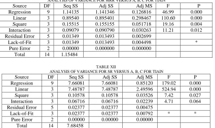
The response surface models are developed in this study with values of R2 say 98.8% and 99.7% for SR and MRR respectively. Furthermore, an R2adj close to the R2 values insure a satisfactory adjustment of the quadratic models to the experimental data. The ANOVA on these models for MRR

and SR of TIAlN is shown in Table 11 and Table 12. It demonstrates that the models are highly significant, as evident from the very low probability of P values in the regression 0.000 and 0.000 for MRR and SR. The lack of fit test describes the variation in the data around the fitted model. If the model does not fit the data well, the lack of fit is not significant.

TABLE XI

ANALYSIS OF VARIANCE FOR MRR VERSUS A, B, C FOR TIAlN

Regression 9 1.14135 1.141346 0.126816 46.99 0.000

Linear 3 0.89540 0.895401 0.298467 110.60 0.000

Square 3 0.15515 0.155155 0.051718 19.16 0.004

Interaction 3 0.09079 0.090790 0.030263 11.21 0.012

Residual Error 5 0.01349 0.013493 0.002699

Lack-of-Fit 3 0.01349 0.013493 0.004498 * *

Pure Error 2 0.00000 0.000000 0.000000

Total 14 1.15484

TABLE XII

ANALYSIS OF VARIANCE FOR SR VERSUS A, B, C FOR TIAlN

Regression 9 7.66081 7.66081 0.85120 179.02 0.000

Linear 3 7.48787 7.48787 2.49596 524.94 0.000

Square 3 0.10578 0.10578 0.03526 7.42 0.027

Interaction 3 0.06716 0.06716 0.02239 4.71 0.064

Residual Error 5 0.02377 0.02377 0.00475

Lack-of-Fit 3 0.02377 0.02377 0.00792 * *

Pure Error 2 0.00000 0.00000 0.00000

Total 14 7.68458

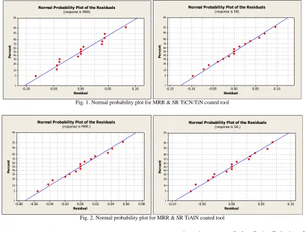
It is usually necessary to check the fitted model to ensure it provides an adequate approximation to the real system. Unless the model shows an adequate fit, proceeding with investigation and optimization of the fitted response surface is likely to give poor results. The normal probability plots for TiCN/TiN of MRR and SR are shown in Figure 1 and normal probability plots for TiAlN of MRR and SR are shown in Figure 2. The data plotted against a theoretical normal

(6)

Residual P e rc e n t 0.10 0.05 0.00 -0.05 -0.10 99 95 90 80 70 60 50 40 30 20 10 5 1

Normal Probability Plot of the Residuals

(response is MRR)

Residual P e rc e n t 0.10 0.05 0.00 -0.05 -0.10 -0.15 99 95 90 80 70 60 50 40 30 20 10 5 1

(response is SR)

Fig. 1. Normal probability plot for MRR & SR TiCN/TiN coated tool

Residual P e rc e n t 0.08 0.06 0.04 0.02 0.00 -0.02 -0.04 -0.06 -0.08 99 95 90 80 70 60 50 40 30 20 10 5 1

(response is MRR.)

Residual P e rc e n t 0.10 0.05 0.00 -0.05 -0.10 99 95 90 80 70 60 50 40 30 20 10 5 1

(response is SR.)

Fig. 2. Normal probability plot for MRR & SR TiAlN coated tool

IV CONCLUSIONS

The objective of this study is the development of response surface design for finding the significant factor affecting in CNC turning on AISI1040. The following conclusions are made through this work.

 The response surface models were developed from the experimental data and predicted values are fairly close. The lack of fit test describes the variation in the data around the fitted model. The lack of fit is not significant. The normal probability plots are departure from this straight line would indicate a departure from a normal distribution, which is used to check the normality distribution of the residuals.

 The linear effect of depth of cut is significantly affecting the MRR followed by interaction effect of feed and depth of cut. The linear effect of feed is significantly affecting SR followed by linear effect of cutting speed for TiCN/TiN and TiAlN.

REFERENCES

[1] A.E. Diniz, R. Micaroni. (2002), Cutting conditions for finish

turning process aiming: the use of dry cutting, International Journal Machine Tool Manufacture, 42, pp. 899- 904.

[2] G. Boothroyd, W.A. Knight, Fundamentals of machining and

machine tools, CRC Press, Taylor and Francis Group (2006).

[3] D. Biermann, M. Kirschner, K. Pantke, W. Tillmann, and J.

Herper, (2013), New coating systems for temperature monitoring

in turning processes, Surface Coating Technology, 215, pp.376-380.

[4] L. Bruce, T. David, A. Stephenson, J. Richard, A. Furness, J.

Albert and J. Shih, (2014), Minimum Quantity Lubrication in Automotive Power train Machining, Sixth CIRP International Conference on High Performance Cutting, Procedia CIRP, 14, pp.523–528.

[5] A. Devillez, G. Le Coz, S. Dominiak, D. Dudzinski, (2011), Dry

machining of Inconel 718, work piece surface integrity, Journal of

Material Processing Technology,211, pp.1590-1598.

[6] K. Chandrasekaran, P. Marimuthu, K. Raja, (2012), CNC turning

on AISI410 with single and nano multilayered coated carbide tools under dry conditions, Journal of Engineering and Technology, 2(2), pp. 75-81.

[7] D. A. F. Orrego, L. B. V. Jimenez, J.D.E. Atehortua, D. M. L.

Ochoa, Effect of the variation of cutting parameters in surface integrity in turning processing of an AISI 304 austenitic stainless steel, Proceedings of First International Brazilian Conference on Tribology, 24-26 November 2010, pp.434-446.

[8] G. Ugrasena, H. V. Ravindra, G. V. Naveen Prakash, R.

Keshavamurthy, (2014), Process Optimization and Estimation of Machining Performances Using Artificial Neural Network in Wire EDM, Procedia Materials Science, 6, pp. 1752–1760.

[9] Shukry H. Aghdeab, Laith A. Mohammed, Alaa M. Ubaid,

(2015), Optimization of CNC Turning for Aluminum Alloy Using Simulated Annealing Method, Jordan Journal of Mechanical and Industrial Engineering, 9(1), pp.39-44.

[10] George E. P. Box, and Norman R Draper. Empirical

model-building and response surfaces, A Wiley-Interscience Publication. 1st edition, Canada John Wiley and Sons, (1987).

[11] K. Chandrasekaran, P. Marimuthu, K. Raja, (2013), Prediction