Abstract— Piping systems in refineries and petrochemical plants are exposed to corrosive environment causing various types of degradation mechanisms. One of the damage mechanisms experienced is gradual wall thinning that causes the pipe to leak. S ince the piping systems carry hydrocarbons or other process fluids, the presence of small leak may lead to a hazardous situation. Therefore, proper inspection and maintenance of these systems is essential for maintaining a safe and continuous operation. Risk-based inspection (RBI) strategy has been adopted to establish the inspection strategy for piping systems where the strategy is based on risk calculated. Risk is defined as the product of the probability of failure and its consequences of failure.
Assessing the failure probability for piping systems in RBI approach typically follows the guideline by American Petroleum Institute (API 581) where the method is deterministic. This study explores the available probabilistic analysis techniques in estimating the piping failure probability, namely, degradation analysis and first-order reliability method (FORM). The objective of this paper is to estimate the pipes failure probability using these two techniques where both models require different input data. Degradation analysis only uses the pipe wall thickness data that are usually being collected during inspection for pipes subject to wall thinning. Conversely, FORM model requires data on material properties and physical geometric of the piping system to estimate the failure probability. The failure probability estimated by these two techniques are then compared and discussed. The results showed that the degradation analysis is more conservative compared to FORM.
Index Term— Piping Reliability, Degradation Analysis, First-Order Reliability Method, Risk-based Inspection
I. INTRODUCTION
ONE of the most important structural elements in refineries and petrochemical plants is piping systems . According to the statistics, the highest percentage of structural elements in those plants is piping systems when compared to other equipment [7]. In general, piping systems in refineries and petrochemical plants are exposed to corrosive environment due to the presence of water, minerals and the stress concentration and this usually leads to various types of degradation mechanisms. Guidelines on the damage mechanisms that affect fixed equipment and piping systems in refineries were issued by American Petroleum Institute, API 571 [2].
One of the most common damage mechanisms experienced by piping systems is wall thinning which can be due to many reasons, including flow-accelerated corrosion [13, 26] and
erosion-corrosion [25]. Gradual wall thinning can cause the pipe to leak or in the worst scenario, the pipe may rupture. Since the piping systems carry hydrocarbons or other process fluids, the presence of small leak or rupture in lines may lead to a hazardous situation. Hence, to maintain a safe and continuous operation, proper inspection and maintenance of these piping systems is crucial.
Unfortunately, regulatory requirements on piping safety and inspection interval is lacking when compared to pressure vessels where the inspection interval requirement is clearly documented. American Petroleum Institute does provide a guideline on the inspection interval of three categories of piping systems based on fluid content in piping or the half remaining life [3]. However, this is generally insufficient as the actual conditions of the piping are not considered and thus, the possible failure of the piping is usually not quantified. According to Giribone and Valette [12], failure probability is the main driver for scheduling periodical inspections in risk-based inspection (RBI) approach. The traditional method to quantitatively assess the failure probability is through statistical analysis of failure data from which a lifetime distribution is developed. This is applicable if there are enough failure data available which is rarely the case for piping failures.
What usually available is a collection of degradation data which is the measurements of equipment wear taken during inspection. This measurement data is used to assess damage before any catastrophic failure occurs. For piping systems that are susceptible to wall thinning degradation mechanism, the wall thickness measurements are usually collected. In this case, degradation analysis is useful for the analysis of failure time distributions in reliability studies [4, 20].
Another technique to assess the failure probability is using first-order reliability method (FORM), a computational method for structural reliability. Unlike degradation analysis that uses only the actual condition data of the piping system where in this study, the wall thickness are considered, FORM model requires more data such as material properties and physical geometric of the piping system to estimate the failure probability.
This study aims to model the pipe failure probability using degradation analysis and FORM, to be further used in RBI strategy in establishing the inspection interval for piping system. The guideline by American Petroleum Institute, API 581, provides the method to assess the failure probability [1];
Comparative Study between Degradation
Analysis and First Order Reliability Method for
Assessing Piping Reliability for Risk-Based
Inspection
however, the assessment is deterministic and does not incorporate the uncertainties in the values of the parameter. The objective of this paper is to estimate the p ipes failure probability using the abovementioned probabilistic techniques, degradation analysis and FORM. The failure probability approximated by these two techniques are compared and discussed. A brief description of both methods will also be discussed.
II. RISK-BASED INSPECT ION
Over the past few decades, the strategies in inspection and maintenance have progressed from the primitive breakdown maintenance to the more sophisticated strategies like condition monitoring and reliability centered maintenance. One of the reasons for the paradigm shift was motivated by the need to implement new maintenance strategies which would increase the effectiveness and profitability of the business. Another link in this chain of progress has been recently added by the introduction of a risk-based approach to inspection and maintenance. Risk-based approach to inspection and maintenance has been suggested as a new vision for asset integrity management[15, 16, 17].
RBI has been an industry standard for prioritizing inspection of static equipments aiming at identifying, characterizing, quantifying and evaluating the likelihood of the loss caused as a result of the occurrence of a specific event. In RBI strategy, risk is used as a criterion to prioritize inspection tasks for t he systems. Risk is defined as the product of the probability of failure and its consequence of failure. The methods to assess risk range from qualitative to quantitative where qualitative approaches are based primarily on expert judgment and specific plant experience and quantitative approaches are based on statistical calculations using large historical databases.
The techniques to estimate probability of failure also varies from qualitative to quantitative. In qualitative failure probability assessment, the probability of failure is primarily based on engineering judgments made by experts. The failure probability is described using terms such as very unlikely, unlikely, possible, probable or highly probable where subjective scores are assigned to different factors which are thought to influence the probability of failure [8, 9, 10]. In a fully quantitative failure probability assessment, the most straightforward approach is to obtain statistical estimates of equipment failure rates based on data collected such as failure data [11, 16, 21, 25]. The main problem with statistical analysis is that it is often difficult to collect enough data to estimate the parameters of the statistical distribution. Another difficulty is to obtain an appropriate statistical d istribution of the data and to justify the underlying assumptions of the selected distribution. When such assessments are undertaken, justification of the relevance of the underlying data and chosen model is usually necessary.
Reliability assessment based on failure data is often hindered by the lack of observed or recorded failures. In this case, inspection data is typically collected. Inspection data are a collection of degradation data which is the measurements of equipment wear usually taken during the inspection period. For piping systems that are susceptible to wall thinning degradation mechanism, the wall thickness measurements are usually collected. In this case, degradation analysis is useful
for the analysis of failure time distributions in reliability studies [4, 20].
III. DEGRADAT ION ANALYSIS
Degradation analysis involves the measurement and extrapolation of degradation data that can be directly related to the presumed failure [22]. A level of degradation at which a failure is said to have occurred needs to be defined first. The use of the term failure in this context is defined as when the wall thickness reaches the minimum wall thickness allowed. To perform degradation analysis, the extrapolation can be done using the one of the following models:
Linear model yaxb
Exponential model ybeax Power model ybxa
Logarithmic model yaln
x bwhere y represents the degradation, x represents time and a
and b are model parameters to be solved for. Once the model parameters have been estimated for each sample i, a time xi
can be extrapolated, which corresponds to the defin ed level of failure y. The computed xi can now be used to as the mean time-to-failure data for the life data analysis.
Life data analysis is one of the well-known engineering tools for analyzing failure data and becomes the tool of choice for many reliability engineers. The technique has applications in a wide range of industries such as military, automotive, electronics, composites research, aerospace, electrical power, nuclear power, dental research and advertising . There are several lifetime distribution models that have been successfully served as population models for failure data such as exponential, Weibull, lognormal, gamma and many other distributions. In this study, the mean time-to-failure data is fitted to the Weibull distribution.
In life data analysis, the mean life is determined by analyzing time-to-failure data. For the case of the piping reliability, the time-to-failure data are extrapolated from degradation analysis. The cumulative density function fo r Weibull distribution is
t t
F 1 exp
where F
t represents the cumulative density function oftime-to-failure i.e. probability that a failure occurs before time t and t is the time-to-failure. The distribution is characterized by two parameters, the scale parameter and
the shape parameter . The value of the parameter
identifies the mode of failure rate. For example, < 1 means decreasing failure rate, = 1 indicates random failure
(constant failure rate) and > 1 describes wear-out failure (increasing failure rate). The scale parameter is defined as
Fig. 1. Degradation analysis framework for piping reliability estimation
IV. FIRST-ORDER RELIABILIT Y MET HOD
First-order reliability method (FORM) has been applied to assess the system reliability with corrosion defects, for example, in pipelines [14, 23, 24].
The failure behavior of the structure is described by a failure function g(x), depending on basic random variables
x xn
x 1,..., which denote applied loads and structural resistance parameters such as dimensions and material properties. By definition,g(x) < 0 implies failure, whereas no failure occurs with g(x) > 0. g(x) = 0 defines the so-called
failure surface, a hyper-surface in the n-dimensional space of the basic variables. The failure surface separates the failure domain F (withg(x)< 0) and the safe domain (g(x) > 0).
The failure probability Pf can be calculated as the probability
content of the failure domain F:
n
n nF
f f x f x x x
P
1 1 ... d 1...d (1)where fi
xi represents the probability densities of therespective basic variables xi, which for the sake of simplicity are assumed to be stochastically independent.
In this study, the failure function is defined as the difference between the pipe failure pressure Pf and the pipe
operating pressure Pop as stated:
op f P P x g( )
Two failure pressure models are used to determine the failure probability namely modified B31G [25] and Shell 92 [6]. The modified B31G failure pressure model is defined as
1 ) ( 85 . 0 1 ) ( 85 . 0 1 ) 95 . 68 ( 2 M t T d t T d D t YS Pf where 50 for 3 . 3 032 . 0 50 for 003375 . 0 6275 . 0 1 2 2 2 2 2 2 2 Dt L Dt L Dt L t D L Dt L M
The Shell 92 failure pressure is defined as :
1 ) ( 1 ) ( 1 8 . 1 M t T d t T d D t
Pf UTS
where Dt L M 2 805 . 0 1
)
(
T
d
= depth of corrosion YS= Yield strength (MPa)UTS= Ultimate tensile strength (MPa) t= Thickness of the pipe (mm)
D= Outer diameter of the pipe (mm) CR= Corrosion rate (mm/yr)
op
P = Operating pressure (MPa)
T= Time of inspection (year)
L= Axial length of corrosion defect (mm)
In this study, it is assumed that the depth of corrosion is
T
CR
t
T
d
(
)
0
.
20
Figure 2 represents the FORM framework for assessing the failure probability.
Fig. 2. FORM framework for piping reliability estimation
V. CASE ST UDY
The pressurized heavy water reactor (PHWR) outlet feeder piping system is taken as a case study [25]. The 70-mm diameter feeder pipes are made of carbon steel A106GrB and are subjected erosion-corrosion damage mechanism. Wall thickness data were simulated based on the mean and standard deviation, as shown in Table I. Both parameters are assumed to follow normal distribution. It is also assumed that the wall thickness data were taken at six different locations.
TABLE I
Pipe parameters [25]
Parameters Mean Standard deviation
T hickness of the pipe (mm) 7 0.385
Corrosion rate (mm/yr) 0.051 0.122
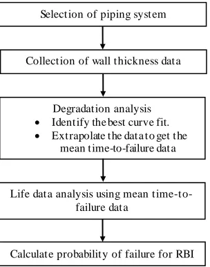
Selection of piping system
Collection of operating data
Calculate failure probability using FORM based on standard models for
RBI Select ion of piping system
Collection of wall thickness data
Degradation analysis
Identify the best curve fit.
Extrapolate the data to get the mean time-to-failure data
Life data analysis using mean time-to-failure data
A. Degradation Analysis
Degradation analysis was performed on the simulated data for each different location where a linear model is assumed to describe the relationship between the wall thickness and time. Using Regression in Microsoft Excel Analysis Tools, the model parameters a, the slope or the corrosion rate and b, the intercept are established. Table 2 shows the equation of the linear model for each location. All locations show a strong relationship between the two variables, time and wall thickness, with the R-squared is more than 0.70. Using the linear model, the wall thickness data was extrapolated to the time when the presumed failure may occur. Here, the failure is defined as when the wall thickness reaches 50% of the wall thickness which is 3.50 mm. The time-to-failure data for each location is also found in Table II.
TABLE II
Linear regression and t ime-to-failure data
Location Linear Equation R-squared T ime-to-Failure (in year) 1 y0.033x6.938 0.7205 103.537 2 y0.058x7.041 0.9765 61.154 3 y0.051x7.056 0.7994 69.768 4 y0.051x7.008 0.8142 69.078 5 y0.037x6.966 0.8836 93.157 6 y0.065x7.078 0.9052 54.899
The next step is to construct a lifetime distribution using Weibull distribution for the estimated time-to-failure data with the assumption that all locations experienced the same conditions. The Weibull cumulative distribution function for the data can be expressed as follows:
093 . 4
922 . 82 exp
1 t
t F
where ttime in years. The shape parameter and scale parameter for the Weibull distribution was found to be
4.093 and 82.922, respectively. This function now can be used to predict the reliability of the piping system at any point time.
B. First-Order Reliability Method
To assess the failure probability using FORM, the following parameters are used as tabulated in Table III.
TABLE III
Parameter for limit-state function with mean and coefficient of variance [25]
Symbol Parameters Mean Variance
YS Yield strength (MPa) 358 25
UTS Ultimate tensile strength (MPa)
455 32
t T hickness of the pipe (mm) 7 0.148
D Outer diameter of the pipe (mm)
72 1.5
CR Corrosion rate (mm/yr) 0.051 0.015
o
P Operating pressure (MPa) 8.7 0.9
T T ime of inspection (year) 30 (constant) L Axial length of corrosion
defect (mm)
300 (constant)
FORM model was built using Microsoft Excel and Visual Basic for Application [18, 19, 27]. The reliability index was obtained by calling Excel’s built-in optimization program,
Solver, with the objective function to minimize the reliability index subject to the constraint that the limit-state function,
g(x) = 0. The probability of failure is then calculated.
VI. RESULT S AND DISCUSSIONS
A case study of feeder piping system is analyzed. Note that for degradation analysis, inspection data in term of wall thickness were used for the analysis whereas for FORM method, the data on pipe material properties and operating parameter were used to assess the probability of failure. The average corrosion rate in degradation analysis was 0.049 mm/year which is comparable to 0.051 mm/year used in FORM analysis. However, the variance of the corrosion rate for degradation analysis is very much smaller with 0.000149 compared to 0.015 used in FORM. The difference might be due to the method in estimation the corrosion rate where in FORM analysis, the corrosion rate was estimated using empirical model as explained in [25].
In FORM analysis, defect depth of 20% of wall thickness was assumed as the initial corrosion depth. A limit state function was defined for a pipe subject to corrosion mechanism that causes wall thinning. The reliability index and the probability of failure were evaluated for various values of inspection period. Based on the probability values, the categorization of failure probability in severity classes has been formulated. Table IV shows the range of failure probabilities and their categories.
TABLE IV
Failure probability categories [1]
Range Like lihood C ate gory
1 10-4 to 1.0 5 Very high
1 10-5 to 1 10-4 4 High 1 10-6 to 1 10-5 3 Medium
1 10-8 to 1 10-6 2 Low
< 1 10-8 1 Very low
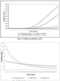
The plots of the failure probability and the reliability index against inspection time are presented, as shown in Figure 3 and 4, to draw the inferences. The graphs can be used as a guide in setting an effective inspection strategy. It is observed from the failure probability generated for the first 10 years for both methods are almost the same. However, after the first 10 years, the probability of failure for FORM model (both B31G and Shell 92) increases exponentially, whereas, for degradation analysis technique, the probability of failure increases gradually at a slower rate. Since > 1 for Weibull
0.00 0.02 0.04 0.06 0.08 0.10 0.12 0.14 0.16 0.18 0.20
1 2 3 4 5 6 7 8 9 10 111213 14 1516 1718 1920 21 22 23 2425 2627 28 29 30
Tim e (in year)
P
ro
b
a
b
il
it
y
o
f
fa
il
u
re
Degradation analysis Shell 92 B31G
Fig. 2. Failure probability plot
Fig. 3. Reliability index vs. exposure time
The failure probabilities and the likelihood categories were calculated at the end of the 30 years of service life as shown in Table 5. The reliability index equations for each method are presented in Table V.
TABLE V
Reliability index equations
METHOD RELIABILITY INDEX EQ UATION
Β(T) AT 30 YEAR S
FAILURE PROBABILIT
Y AT 30 YEARS
LIKELIHOO D CATEG ORY
Degradatio n Analy sis
2.2567 0.0120 5
FORM using B31G
1.1946 0.1161 5
FORM using Shell 92
0.9280 0.1767 5
VII. CONCLUSION
In this paper, the failure probability assessment models based on degradation model and first-order reliability method were developed and applied to estimate the failure probability of wall-thinned feeder piping systems. This study was needed to establish inspection program for piping systems based on the quantitative risk assessment. Both models are compared and the following key findings have been derived:
Degradation analysis is conservative because it appears that the pipe might not fail for longer exposure time. Even if it appears that it has not failed, it may not be safe to use
it. For safety reasons, it would be wise for the pipe to be repaired or replaced.
The FORM results are well comparable with the results available in the literature.
ACKNOWLEDGMENT
The authors gratefully acknowledge all reviewers fo r their valuable suggestions for enriching the quality of the paper. The support of Universiti Teknologi PETRONAS is greatly acknowledged.
REFERENCES
[1] American Petroleum Institute. (1996). Base Resource Docum ent on Risk-Based Inspection. API Publication 581.
[2] American Petroleum Institute. (1997). Damage m echanism s that affect fixed equipment and piping system s in refineries. API Publication 571. [3] American Petroleum Institute. (2001). Piping Inspection Code. API
Publication 570.
[4] Bae, S.J., Kuo, W. and Kvam, P.H. (2007). Degradation models and implied lifetime distributions. Reliability Engineering and System s Safety , 92, 601-608.
[5] Caleyo, F., Velazquez, J.C., Valor, A. and Hallen, J.M. (2009). Markov chain modeling of pitting corrosion in underground pipelines. Corrosion Science , doi: 10.1016/j.corsci.2009.06.014.
[6] Caleyo,F., Gonzalez, J.L. and Hallen, J.M. (2002). A study on the reliability assessment methodology for pipelines with active corrosion defects. International Journal of Pressure Vessels and Piping , 79, 77-86.
[7] Chang, M., Chang, R. Shu, C. and Lin, K. (2005). Application of risk based inspection in refinery and processing piping. Journal of Loss Prevention in the Process Industries , 18, 397-402.
[8] Dey, P. (2001). A risk-based model for inspection and maintenance of cross-country petroleum pipeline. Journal of Quality in Maintenance Engineering , 7 (1), 25-41.
[9] Dey, P. (2004). Decision support system for inspection and maintenance: A case study of oil pipelines. IEEE Transactions on Engineering Managem ent , 51 (1), 47-56.
[10] Dey, P.K., Ogunlana, S.O. and Naksuksakul, S. (2004). Risk -based maintenance model for offshore oil and gas pipelines: a case study. Journal of Quality in Maintenance Engineering , 10 (3), 169-183. [11] Fleming, K. (2004). Markov models for evaluating risk -informed
in-service inspection strategies for nuclear power plant piping systems. Reliability Engineering and System Safety , 83, 27-45.
[12] Giribone, R. and Valette, B. (2004). Principles of failure probability assessment (PoF). International Journal of Pressure Vessels and Piping , 81, 797-806.
[13] Hales, C., Stevens, K.J., Daniel, P.L., Zamanzdeh, M. and Owens, A.D. (2002). Boiler feedwater pipe failure by flow-assisted chelant corrosion. Engineering Failure Analysis , 9, 235-243.
[14] Juang, C. H., Fang, S. Y and Khor, E. H. (2006). First -order reliability method for probabilistic liquefaction triggering analysis using CPT . Journal of Geotechnical and Geoenvironmental Engineering , 132 (3), 337-350.
[15] Khan, F.I. and Haddara, M.M. (2003). Risk-based maintenance (RBM): a quantitative approach for maintenance /inspection scheduling and planning. Journal of Loss Prevention in the Process Industries , 16, 561-573.
[16] Khan, F.I., Haddara, M.M. and Bhattacharya, S.K. (2006). Risk -based integrity and inspection modelling (RBIMM) of process components/system. Risk Analysis , 26 (1), 203-221.
[17] Krishnasamy, L.,Khan, F. and Haddarra, M. (2005). Development of risk-based maintenance (RBM) strategy for a power-generating plant. Journal of Loss Prevention in the Process Industries , 18, 69-81. [18] Low, B. K. and T ang, W. H. (2007). Efficient spreadsheet algorithm for
first-order reliability method. Journal of Engineering Mechanics , 133 (12), 1378-1387.
[19] Low, B. K. and T ang, W. H. (2004). Reliability analysis using object -oriented constrained optimization. Structural Safety , 26, 69-89. [20] Meeker and Escobar. (1998). Statistical m ethods for reliability data.
New York: Wiley.
[22] ReliaSoft Corporation. (2006). Life Data Analysis. T ucson, AZ: ReliaSoft Publishing.
[23] Santosh, Vinod, G., Shrivastava, O.P., Saraf, R.K., Ghosh, A.K. an d Kushwaha, H.S. (2006). Reliability analysis of pipelines carrying H2S for risk based inspection of heavy water plants. Reliability Engineering and System Safety , 91, 163-170.
[24] T eixeira, A. P., Soares, C. G., Netto, T . A. and Estefen, S. F. (2008). Reliability of pipelines with corrosion defects. International Journal of Pressure Vessels and Piping , 85, 228-237.
[25] Vinod, G., Bidhar, S.K., Kushwaha, H.S., Verma, A.K. and Srividya, A. (2003). A comprehensive framework for evaluation of piping reliability due to erosion-corrosion for risk-informed inservice inspection. Reliability Engineering and System Safety , 82, 187-193.
[26] Yuan, X. X., Pandey, M. D. and Bickel, G. A. (2008). A probabilistic model of wall thinning in CANDU feeders due to flow-accelerated corrosion. Nuclear Engineering and Design , 238 (1), 16-24. [27] Zhao, Y. and Ono, T . (1999). A general procedure for first/second-order