S O F T W A R E
Open Access
Strand: scalable trilateration with
Node.js
Konstantinos Tserpes
1*, Maria Pateraki
2and Iraklis Varlamis
1Abstract
This work reports on the development details and results of an experimental setup for the localization of the attendants of a music festival. The application had to be reporting in real-time the asymmetric crowd density based on the Received Signal Strength Indicator (RSSI) between the attendants’ smartphones and an experimental installation of 24 WiFi access points. The impermanent nature of the application led to the implementation of a cloud-based solution, called “STRAND”. STRAND is based on Node.js components, which communicate through websockets, collect, process and exchange data and continuously report the produced information to the end-user. To cope with the near real-time requirements, and the volatility of the crowd concentration density, STRAND
horizontally scales the trilateration component, i.e. the component that estimates the user location based on distance measurements. STRAND was tested during the festival days in July 2018 and the results show a system that copes with very high loads and achieves the temporal and accuracy requirements the were set.
Keywords: Autoscaling, IaaS, NodeJS, Websockets, RSSI, Localization, Trilateration
Introduction
A music festival in Germany concentrates dozens of thou-sands of visitors within a mid-July weekend every year. At peak times it reaches almost 150,000 visitors. The organizers would like to have a bird’s eye view of the con-centration of the visitors in the area of the festival, so as to identify situations of emergency and to swiftly adapt their risk mitigation plans such as the evacuation plans of the area. This resulted to the need for a heatmap visualization that depicts the crowd concentration density, in the map, in near-real time (i.e. at 1 min intervals). This implies that once the position information is collected, by an installa-tion of sensors, it has to be processed and reported to the organizers’ dashboard within 1 min.
During the festival days, the large crowd is concentrated in a relatively confined space. This concentration leads to a high contention ratio of the effective mobile telecommu-nication bandwidth practically rendering it useless. The automatic detection of crowd concentration in near-real time is a critical yet challenging task for the organizers. Using image analysis techniques for this task, suffers from
*Correspondence:[email protected]
1Department of Informatics & Telematics, Omirou 9, GR17778 Tavros, Greece
Full list of author information is available at the end of the article
lack of computational resources to handle the increased complexity and results in an increased installation cost. Also, such methods do not perform well in all conditions (e.g. in low light) and can hardly avoid counting the same person multiple times. Techniques that transmit the GPS signal of users’ devices via a smartphone app are energy and bandwidth consuming. As a result, the use of the festi-val official mobile app for collecting position data from the devices’ GPS receiver is not an option since the app will have to compete for the limited bandwidth with popular mobile apps such as Instagram, Facebook, Twitter, etc.
The restrictions of visual techniques in such environ-ment and the high energy consumption of embedded GPS sensors in smartphones and the frequent loss or erro-neous GPS signal due to unavoidable obstructions, i.e. trees, buildings, etc., leave space for passive techniques, which take advantage of the pervasive availability of WiFi infrastructure and allow effective localisation and crowd concentration estimation in outdoor as well as in indoor scenarios.
In order to exert the WiFi-based outdoor localization we deployed a number of Raspberry Pi devices which are con-figured to operate as open WiFi access points (APs). The mobile devices of the visitors, with their WiFi transceiver activated, would poll continuously for the networks in
their vicinity, exchanging some basic information with the WiFi open access points. The received signal strength indicator (RSSI) could be then used to estimate the dis-tance of the users from multiple access points and then, by a process known as "trilateration", to estimate the position of those users. This is an approach commonly employed in the literature mainly in indoor localization setups.
From a non-functional point of view, the application
needed to be scalable, i.e to be able to simultaneously
locate a large number of users, maintaining the near real time (1 min) requirement and ensuring that the cost in resources based on the asymmetric crowd’s density fluc-tuates proportionally to the crowd’s volume at various times.
Also, the application should provide adequate
guaran-tees regarding the users’ location privacy. To deal with
the first issue it was necessary to employ cloud resources and the cloud providers’ API that would enable the auto-matic scaling. For the issue of privacy, as the user location can be correlated with far more personal information related to behavior, mood etc., appropriate encryption was adopted to preserve and guarantee the user loca-tion privacy and anonymity, namely the MAC address of the users’ mobile devices was obfuscated using pseu-doanonymization.
A third requirement was related to theaccuracyof the
location estimation, considering minimum cost for infras-tructure and low number of nodes to obtain an estimate on user location, to avoid delays and performance degra-dation due to packet collision or wrong measurements
[43], an error of 12 meters in terms of 2D accuracy was
permitted by the festival organizers. This requirement is also tightly linked to the previous as this relaxed accu-racy threshold also served as an artificial way to obfuscate the actual users’ positions. Finally, in parallel to the low cost aspect of the application, vendor locking-in should be avoided, as the festival is essentially free and it is rely-ing on volunteers without much expertise on the field of application development.
The experimental setup comprised of 24 operational Raspberry PI devices covering critical areas of the festi-val grounds, including the main entrance/exit, the three main stages, the food and drink stand and the toilets. The devices were deployed in clusters of 3 or 4 with trees, infrastructure and festival facilities often obstructing their line of sight with the attendants. The measurements were collected in an on-site system and then distributed through a satellite link to the cloud-based application pipeline. The federation between the edge nodes, ie. the Raspberry PI devices, and the cloud was orchestrated by a
cloud brokerage platform, called BASMATI ([2,3]).
The research objectives were to implement the cloud-based application that would support the processing of the measurements and provide a near real-time (1 min
intervals) heatmap of the crowd’s concentration density. The low-cost requirement for the application as well as its impermanent nature justified the use of cloud resources and the satellite link instead of an investment in perma-nent resources. The implementation was based on Micro-Service Architecture inspired by a pattern introduced in [36].
The main contributions of this work are:
• an open source software reference implementation, • a cost-efficient, easy-to-deploy, large-scale
localization system,
• a micro-service architecture pattern that allows efficient load balancing on the cloud.
The implementation details of STRAND and the expe-rience from its use during the festival days (July
19-22, 2018), are described in what follows: “Related work”
section provides an analysis of the state of the art that justified the selection of the individual decisions in the
application implementation; “Implementation” section
gives the implementation details including the applica-tion architecture, the components’ funcapplica-tionality and inter-faces, the implementation technology decisions and the key-design characteristics. The evaluation results are
pre-sented in “Evaluation results” section and in Section
Conclusionsthe major conclusions of this work.
Related work
A thorough analysis of the current state-of-the-art in two main distinct domains was conducted prior to the imple-mentation of the application: the localization systems and the cloud load balancing techniques. The selection of tools, technologies and approaches was based on the par-ticular requirements of the application. This analysis is presented in what follows.
Passive sensing localization techniques
The use of image analysis techniques for the estimation of crowd density and person localisation has been pro-posed in the literature. For example, road traffic detection systems are using image segmentation and analysis
tech-niques for processing the signal from road cameras [5],
for the detection and counting of vehicles. In the case
of crowd counting, Crowdnet [6] is a deep CNN trained
to analyse video streams, whereas Convolutional LSTMs
have been proposed in [41] for creating crowd density
maps. An interesting survey on the use of CNN for
single-image crowd counting can be found in [32]. The advantage
thermal cameras or infrared cameras or combinations are used, which also increases the cost of the installation. Finally, visual solutions may have to tackle the problem of blind spots. In the case of a festival, this requires multi-ple cameras to increase coverage and careful position in order to avoid double counting. The latter is avoided by device-based methods that employ the device identify for disambiguation.
A large body of works deal with the problem of local-ization of "blind" nodes by passively sensing WiFi, Blue-tooth or RFID signals. The methods are either device-free [10,14] or device-dependent [40]. In the former case, a set of transmitters and receivers operates in a constant basis and human presence is detected based on changes in the strength of the received signals. In the latter case, users are carrying devices, which transmit WiFi or similar sig-nal and a set of area sensors continuously collect the sigsig-nal and analyse its strength. In such cases, the signal strength is used to detect the distance from each fixed sensor node, and algorithmic approaches, such as trilateration or N-point lateration, are employed for the estimation of the position of the moving signal source.
In fact, the concept appears in multiple works, both in indoor and outdoor localization with the former com-prising the bulk of the works in the literature (e.g. [7, 18,29, 31, 43]). When it comes to outdoor localiza-tion, there is a range of approaches being used so as to determine the location of a node in question. The major-ity of them are relying in measuring the distance of the blind node from a number of fixed-point (anchor) nodes that are part of the same Wireless Sensor Network (WSN) and then employing algorithms to estimate the node’s location. Some common distance measurement meth-ods are angle of arrival (AoA) (e.g. [39]), time of arrival
(ToA) (e.g. [30]), time difference of arrival (TDoA) (e.g.
[42]), acoustic energy (e.g. [38], time of flight (TOF) (e.g.
[16]) and received signal strength indicator (RSSI) (e.g.
[13, 34, 35]). The first three methods require complex
hardware set up, while TOF needs line of sight to effec-tively locate nodes. On the other hand, RSSI-based solu-tions are easy to implement and cost efficient but less accurate due to additional signal attenuation resulting from transmission through big obstacles and severe RSS fluctuation due to multipath fading ([9,24]).
Beyond this range-based technique, other solutions have been presented for outdoor localization such as topographical maps and propagation-prediction tools, as well as statistical modeling, neural networks and particle filters ([23]).
Once the distance of the node in question is known from at least 3 known anchor nodes, the problem is reduced to an overdetermined system. Assuming a linear state space, the system is comprised of at least 3 second-degree poly-nomials expressing the euclidean distances of the node
in question from the anchor nodes. By subtracting them, the polynomial degree is reduced and thus the system is solvable with standard algebraic solutions such as a least squares approximation. This approach was followed by
[25] and it seems to be appropriate in small distances and
near perfect input. In the case of the festival, the dis-tances are large and the natural environment affect the RSSI. Furthermore, if the number of equations increases, i.e. more than 3 anchor points report their inaccurate RSSI with the node in question, the linear least squares solution complexity increases. The alternative is to use a nonlinear least squares fitting approach such as the
Levenberg-Marquardt curve-fitting algorithm ([12]). The
latter is appropriate for real-time operations due to its low complexity, however, the accuracy degrades when the
measuring node’s speed increases([26]).
This work employs an RSSI-based trilateration local-ization algorithm to accurately localize the festival atten-dants’ smartphones. To deal with the near real-time requirements, the Levenberg-Marquardt curve-fitting algorithm was used for the trilateration part, considering the fact that the monitored crowd moves typically in very low speeds.
Cloud computing load balancing
Load balancing is a critical component provided by every public cloud service provider as it allows the application to adapt to load demands dynamically. scaleout and scalein operations are typically employed, allowing the horizontal scaling of the application, i.e. adding new cloud resources (scaleout) and removing them (scalein) at runtime so as to cope with the load. On the other hand, vertical scaling, i.e. adding more "power" to the existing cloud resources for load balancing purposes, is generally more rare (e.g. [33]) due to the high overhead and hard constraints involved in vertical scaling (usually the machines have to be reset). Load balancing in IaaS environments, implies that an application can scale through the addition or removal of Virtual Machines (VM). This is a standard practice in
many applications, including distributed databases [20].
There are various taxonomies for load balancing
strate-gies in the literature (e.g. [1, 22]). Perhaps the most
relevant classifications for STRAND relate to the distinc-tion of applicadistinc-tion-agnostic VS applicadistinc-tion-oriented and dynamic Vs static load balancing strategies.
Practically all major cloud providers are offering
off-the-shelf IaaS solutions for load balancing1 2. In order
for them to maintain a general purpose nature, they are made in a stateful way, i.e. they operate independently of the application characteristics. This is commonly referred to as "load balancing as a service" ([8, 27]). As such,
the load balancing strategy is built on the basis of an infrastructure-related metric, such as the resource utiliza-tion of the processors, or the incoming traffic (requests per second-RPS). These strategies are part of what is referred to as internal and/or HTTP load balancing. There is the option to distribute instances from a regional managed instance group, based on custom-made metrics
using external tools such as Google’s Stackdriver3but this
usually comes at an extra cost.
However, in other cases, the load is defined in terms of application-related metrics, as in distributed data man-agement systems, where the load is dependent on the amount of load/store operations ([21]). In these cases, the Load Balancer must be integrated in the application and be able to invoke the public cloud providers’ API to man-age VMs. This approach also comes at the cost that apart from the deployment of the VM, the Load Balancer needs to instruct the public cloud’s API to install and run the application. This can be done through a startup script that installs and resolves all necessary dependencies and runs the processor’s code or deploys docker files.
This latter approach was selected in the case of this application in order to remove the burden of knowing the public clouds’ concepts from the future application devel-oper. When someone will have to re-run the application, perhaps in a different cloud provider, the idea is to stick to basic devops (expressed in the startup script), which most likely won’t change in the years to come.
In terms of the load balancing strategy, a dynamic approach was followed as opposed to static. In static load balancing, a fixed number of operational proces-sors (or remote nodes) is reserved and the systems use them accordingly. In the case of STRAND, the applica-tion scaled in and out based on some predetermined rules adapting to runtime conditions, and in particular the load itself. In the literature, there is a great number of dynamic load balancing approaches in cloud computing (e.g. [11,15,28]) that apply sophisticated mechanisms to his-torical data so as to predict and cope future loads. In the investigated case, these solutions were not applicable due to the lack of previous knowledge and due to the fact that the systems in the literature are not investigating mobil-ity patterns which were relevant in this case, but different parameters such as e-commerce consumer habits.
Among the two controlling forms in dynamic load bal-ancing algorithms, namely centralized and distributed, STRAND opted for the centralized. In centralized load distribution, a single node in the network is nominated to be responsible for all load distribution in the network. In the distributed approach, many nodes are undertaking the responsibility of sharing the load ([17]). A distributed
solution like [19] would infuse unnecessary complexity
3https://cloud.google.com/stackdriver/
with multiple cloud components needing to be configured to talk to one another.
Implementation The processing pipeline
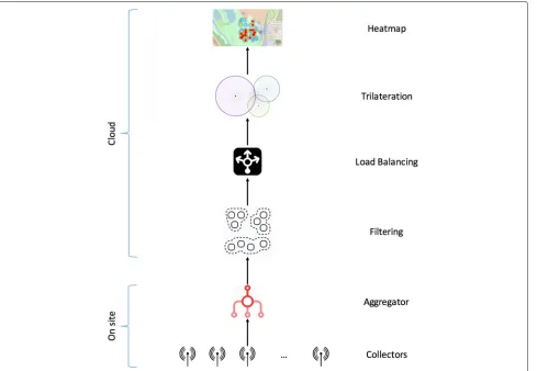
The key concept in this work was to implement a work-flow of standalone components that will process the raw measurements as data streams and will deliver the data for the heatmap visualization. As such, the architecture of the application involves a logical pipeline of a number of components, namely, the data Collectors, the data Aggre-gator, the Clusterer, the Load Balancer, the Trilaterator
(Processor), the Storage and the Frontend (Fig.1). These
are described in detail in what follows.
The first two components in the pipeline are deployed locally on site, as part of a local network and commu-nicating trough standard TCP/IP protocols. The rest of the components are deployed on virtual machines (VM), on cloud resources communicating through websockets. The focus of this paper is to report on the details of the cloud-based part of the application, however for reasons of integrity, the on-site part is also presented.
According to this architecture, the raw WiFi signal mea-surements transmitted by every smartphone in proxim-ity are collected by the Raspberry Pi, using the nexmon
driver (https://github.com/seemoo-lab/nexmon) and a
shell script, which was written for this purpose. Similar
scripts are widely available online4. Each measurement
contains a timestamp and the id of the device that trans-mitted the signal. Data from the Raspberry Pis, which are the local data collectors, are aggregated and anonymized by a physical machine onsite, which stores the data locally and provides an API for accessing them. A cloud-based filtering module is responsible for retrieving data at reg-ular intervals from the onsite machine, aggregating them per uid and sending them to the cloud-based load bal-ancer. The latter is responsible for retrieving data and re-distributing them to micro-services hosted in cloud-based virtual machines for further processing, storage and display. The details for these operations are provided in what follows.
Component functionality
For a better understanding of the role of every component involved in the pipeline, this Section provides a descrip-tion of their funcdescrip-tionality starting from the first item in the pipeline, i.e. the Collectors.
Collectors
The data Collectors are executing the task of sensing for WiFi adapters in their vicinity in fixed time intervals and maintaining a record of their findings locally, in files. They
4
Fig. 1High-level architecture. The STRAND application workflow
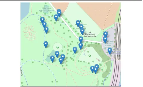
do not perform any other task given that a) their compu-tational capacity is limited, b) their main task of sensing is rather frequent (once every 15”) and c) the fact that they are exposed to adverse weather conditions (outdoors under direct sunlight or rain). The Collectors are deployed in strategically selected positions so as to cover areas of interest and to ensure that some level of overlap exists between their area of coverage (see Fig.2).
Sensing: Operating as WiFi access points with the pre-tense that they are offering an open WiFi access, the Collectors implement a standard communication proto-col with devices (mainly mobile) that have their WiFi transceivers on. Through this process, they are registering 4 main data items for each connected device:
• uid: a unique user id that is in the form of a MAC address, assuming that the connecting, mobile devices are always transmitting the same MAC address. • did: the device id of the Collector device that
collected the data. This field is needed to map the device that collected the signal to a specific location (Lat, Lon pair).
• rssi: the received signal strength indicator in dB. This is needed to estimate the radius upon which the user was detected with the centre being the collector’s device location.
• timestamp: unix time during which the data were generated
Fig. 2Deployment of Raspberry PI access points. The blue markers indicate the positions of the access points
Storing: Each Collector is polling its surroundings for mobile devices in a fixed time interval and writes out the collected information to a locally stored file. One times-tamped file is created for each round of measurements in order to mitigate potential synchronization issues.
Aggregator
The data Aggregator is providing four basic function-alities: data aggregation, initial data filtering, pseu-doanonymization and data access provision to other com-ponents. It is an onsite component running on a physical machine which is part of the Collectors’ network. This machine has access to the internet, thus it bridges the local Collectors’ network to the application cloud resources. It persists the data from the files it collects, organizes them in a relational database and emits them to interested parties.
Data aggregation: The Aggregator, being part of the Collectors’ network, can access their storage and pull the measurement files at fixed intervals. It does so by con-necting to each one of them through SSH and executing a shell script to retrieve the latest data files that it hasn’t retrieved yet. In this way the need for hard synchroniza-tion constraints is lifted with the Aggregator and each of the Collectors executing their operations at independent times and possibly at a different frequency.
Filtering: Occasionally there are reasons to discard cer-tain measurements, e.g. same data are received twice, or the signals are too weak to make any sense. This com-ponent is filtering out measurements that are problem-atic. Also, there are many cases in which the signals are received by external to the application fixed WiFi access points which are consistently trying to register to the open WiFi network. A lookup table can be used here to allow the Aggregator to filter out MAC addresses that belong to such network devices manufacturers or even MAC addresses that persisting measurements’ values.
Pseudoanonymization: To protect user privacy, the Aggregator uses a fixed hash function to transform the uid value from a MAC address to a new, seemingly random, device id. The hash function is deterministic which means that the same input will always result in the same output because it is important to distinguish unique users.
Data access: The Aggregator stores the preprocessed measurements in a db and provides a RESTful API for other components to access it.
Filtering
is to filter the input data structure that it receives from the Aggregator.
Filtering: This functionality clusters messages based on their uid and timestamp, i.e. groups measurements with the same MAC and a timestamp indicating that they were generated within a 1 min time window. The clustering is essentially a two-step process: a) group by uid and b) merge measurements under a single uid and a single timestamp, in particular the last received timestap in the time window. The resulting data structure is comprised of records containing the uid, the timestamp and an array of RSSI values coupled by the Collector’s device id (did) that collected each value, i.e. an array of did, rssi pairs.
Load balancer
The Load Balancer buffers the measurements received by the Aggregator in an internal queue and distributes the load to all connected processor components (Trilatera-tors). Judging from the queue length and the rate that it is evolving, the Load Balancer can request the deploy-ment of more processor components or decommissioning of the excess ones. Assuming the existence of the appro-priate resources, the Load Balancer provides temporal constraint guarantees and it is a central component in the implementation of the scalable application.
Load distribution: This functionality allows to pro-cessor components (Trilaterators) to request and receive measurements to process. The Load Balancer removes the oldest pending object of measurements in the queue for a uid and pushes them to the requesting processor.
Scaling: Simple, demand-based autoscaling rules are adopted. The rationale is that the Load Balancer can iden-tify the need for a new processor component to be added by monitoring the length of its queue periodically. If the rate at which the queue size is increasing exceeds a certain threshold, then the Load Balancer proactively requests the deployment of new processor components. Conversely, if the rate is decreasing, the Load Balancer requests the decommission of the excess processor(s) components. These requests are implemented through the underlying cloud providers’ API (the one to which the processor is deployed). The time that it takes for a new processor to be fully operational and the fluctuating number of measure-ments entering the application both play a detrimental role in the scaling operations, imposing a large number of constraints and exceptions. As such upper and lower thresholds are provided for the queue length. Exceeding those thresholds result in scaling commands to be issued. To avoid new scaling commands to be issued before the previous are completed a cooldown period is provided. Furthermore, the number of VMs that can be spawned at any time is also limited by a value set manually. Equiva-lently, a warm-up period is considered, so as to be able to count the generated instances by increasing them by
one, when the instance actually starts operating. Details on how the various thresholds are selected are discussed in detail in “Evaluation results” section.
Trilaterator
The Trilaterator is undertaking the task of processing measurements that are assigned to it by the Load Balancer and finding the approximate location of the respective user at the given timespan. It is deployed on Virtual Machines and cold or hot deployment is employed based on the end users assigned budget. The particular process-ing that is done is called trilateration and it requests at least three distances of the object in question from an equivalent number of known points, in order to estimate its position. Thus, before the trilateration task, the Trilat-erator is calculating the distance of the user in question from the Collector device by means of the RSSI.
Distance calculation: The distance (dis) is calculated based on the RSSI and the location of the Collector that measured this signal strength. The formula is:
dis=10(Ptx−rssi/10∗plex)
where Ptx is the transmit power of the Collector device
andplexis the path-loss exponent. The context is that the
transmitter and the receiver are rarely placed within a line of sight and that the signal propagation model needs to consider the environment within the transmission takes
place as well as the power it is transmitted [25]. This
general purpose formula considers these two parameters. The default transmit power for DD-WRT based routers is between 70mW or 18.5dBm. Also, as a rule of thumb the path-loss exponent receives the following values: 2 for free space, 2.7 to 3.5 for urban areas, 3.0 to 5.0 in suburban areas and 1.6 to 1.8 for indoors when there is line of sight to the router. For the particular experiment, it was set to 2.5.
Trilateration: Since the Collector’s devices are in fixed points, we can employ a simple lookup table and the did of the Collector’s device to get the approximate location of the Collectors in GPS coordinates. Knowing the distances fromn(n> 2)fixed points allows us to estimate the user
location in the form oflat,loncoordinates.
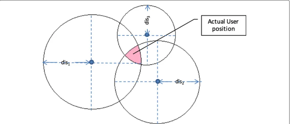
In a perfect situation the rationale behind trilateration would be the following: For each user i and Collector device j there is a pairlocj,disij that defines a sphere of
radiusdisij around locationlocj and the user may lie in
In reality, there are multiple errors that are infused by various systems along the way, including errors in mea-suring the RSSI, inaccurate GPS coordinates of the Collec-tors, erroneous calculation of the distance, etc. Therefore, the spheres may not always intersect, or the intersection
may commonly lead to an area rather than a point (Fig.3).
Selecting any point from the intersection area will result in a declination from the expected values for at least two of the measurements, i.e. the selected point will not be on at least two of the circles. The key point is to identify thelat, lonpair for the user within the intersection area that minimizes this declination. A solution for this prob-lem is to find the user position that will minimize the sum of squares of this declination. This method is called least square and it is commonly used in data fitting problems like the one at hand. In fact, we want to identify the func-tion f which maps the user locafunc-tion (Yi) to the {loc,dis} pair (Xi) of thei−thCollector from a set ofm, or in other wordsYi=f(Xi),i=1. . .m. The evaluation of this func-tion for every Collector will give a residualri, therefore the point is tominimizemi=1r2i.
This problem is solved using the Levenberg-Marquardt algorithm as it is implemented in the trilat package (https://www.npmjs.com/package/trilat).
Storage
The Storage component provides a RESTful API enabling other components to persist user locations to its database and at the same time to access the data.
Persisting: An API allows a client to "push" tuples of
the form of uid, lat, lon, timestamp to the database.
Accessing: An API allows a client to "pull" tuples of the abovementioned format in a stateful, synchronized
way, allowing the querying of the database using multiple criteria.
Frontend
The Frontend is an HTML-based web client that retrieves data from the Storage and depicts it in heatmap visualiza-tion in real time.
Data retrieval: A timed AJAX request is using the Storage API to retrieve data.
Visualization: Using the Leaflet Javascript library (https://leafletjs.com), the Leaflet.heat extension (https:// github.com/Leaflet/Leaflet.heat) and Openstreetmap (https://www.openstreetmap.org/), the Frontend chro-matically depicts the concentration density of users in various locations of the festival area within consequent timespans.
Interfaces and data formats
The basic mode of communication between the cloud-based components is implemented through websockets. Each component maintains a websocket interface for its counterpart for the purpose of data exchange. Depending on the situation the data may be “pushed” or “pulled” (sent after request) from one component to another.
The following subsections provide an overview of the inputs/outputs of the components in terms of data exchange.
Collector
As already stated, the Collectors do not expose any inter-face, rather they allow predefined components to pull their data through SSH.
Input:WiFi signals
Output:raw data files, timestamped. An example mea-surement from one Collector looks like this:
{
" d i d ": " r a s p b e r r y p i−5" , " u i d ": 1 2 3 4 5 7 ,
" r s s i ": −74 ,
" timestamp ": 1532267012 }
Aggregator
The Aggregator pulls the data from the Collectors in a synchronized way, performs some basic processing, stores them and then exposes them through a standard RESTful API.
Input:the output of the Collectors
Output:the same as the input but in arrays grouped by the did. E.g.
{
" d i d ": " r a s p b e r r y p i−5" , " r e c o r d s A r r a y ": [
{
" u i d ": 1 2 3 4 5 7 , " r s s i ": −74 ,
" timestamp ": 1522919784 } ,
{
" u i d ": 1 2 3 4 5 7 , " r s s i ": −76 ,
" timestamp ": 1522919785 } ,
{
" u i d ": 1 2 3 , " r s s i ": −83 ,
" timestamp ": 1522919787 } ,
] }
Filtering
The Filter pulls the data from the Aggregator, orders them based on their uid and timestamp and pushes the new structures to the Load Balancer. It uses standard HTTPS requests towards the Aggregator and exposes a websocket interface towards the Load Balancer.
Input:The output of the Aggregator
Output:An array of objects, each containing all the col-lectors’ measurements rssi, did for a specific user within a specific timespan (defined by a timestamp, commonly the time that the timespan finishes).
[ {
" u i d ": 1 2 3 4 5 7 ,
" timestamp ": 1 5 2 2 9 1 9 7 8 5 , " s i g n a l A r r a y ": [
{
" d i d ": " r a s p b e r r y p i−5" , " r s s i ": −76 ,
} , {
" d i d ": " r a s p b e r r y p i−8" , " r s s i ": −81 ,
} , {
" d i d ": " r a s p b e r r y p i−9" , " r s s i ": −79 ,
} , ] , } , . . . ]
Load balancer
The Load Balancer receives the measurements in batches from the Filter in a fixed interval (1 min). Then it stores it in its local FIFO queue and distributed one object at a time, to each connected Trilaterator. The communication protocol between the Load Balancer and the Trilaterator is the following:
• Listen for new Trilaterators
• Accept new Trilaterator connections
• Expect a "status":"ready" message from a Trilaterator • Remove the oldest measurement in the queue and
send it to the Trilaterator that issued the "ready" status message
This allows for a flexibility in adding or removing new Trilaterators without the Load Balancer having to know anything about it nor about their status.
Input:The output of the Filter in batches (in an array)
Output:The oldest object from the queue where the Filter batches are stored
Trilaterator
The Trilaterator retrieves data from the Load Balancer through a websocket client according to the previously mentioned protocol. It uses those data to calculate the position of the user. Then it creates a new data structure that includes the uid, timestamp, lat, lon and pushes it through another websocket to the Storage component.
Input:The output of the Load Balancer
Output:A message containing the uid, timestamp, lat, lon, like the following:
{
" u i d ": 1 2 3 4 5 7 ,
" timestamp ": 1 5 2 2 9 1 9 7 8 5 , " l a t ": 4 8 . 9 9 9 1 7 ,
Storage
The Storage component exposes a websocket server for persisting and another for accessing the data. Through the websocket, it can enable a stateful communication with the client, i.e. every time the client sends a particu-lar command, the Storage responds by sending messages pertaining to the latest fixed time interval, i.e. fetches only new messages, starting from where it finished during the previous call.
Input:The output of the Trilaterators
Output:An array of objects in the same format as in the input
Frontend
The Frontend implements a websocket client that pulls data from the Storage and visualizes them, also in an animated way, like a timelapse.
Input:The output of the Storage
Output:
-Underlying technologies and deployment plan
The cloud-based components (Filtering, Load Balancer, Trilaterator and the Storage) are all based on open-source technologies. The components are deployed in a Node.js framework in independent virtual machines, using npm packages such websocket, mysql, forever, tri-lat and @google-cloud/compute. The Storage maintains the data in a standard MySQL database. The Frontend is based on client-side technologies, and in particular HTML, CSS and Javascript (vanilla) as well as Javascript libraries such as Leaflet.Heat.
Node.js is selected as a technology because:
• it is lightweight in comparison to the use of application containers
• it is non-blocking which is critical for the case of the Load Balancer, allowing at the same time to avoid the hassle of dealing with threads
• it is simple passing from front-end to back-end development since both are based on Javascript • it achieves good response times and throughput in
the backend in comparison to other server-side technologies
The communication between components is achieved mainly through websockets. Websockets are appropriate for bi-directional communication and data streams trans-fer, especially when there a many small object like in this case.
The scalability is achieved through the Node.js client
for the Google Compute API (https://www.npmjs.com/
package/@google-cloud/compute). A scalability engine with a simple scale in/out/back interface was imple-mented that allows the creation of new VM instances on Google Cloud and the deployment and execution of the
application code as a startup script. The scalability engine was stateful, maintaining the list of created instances and details about their state. This kind of information was useful once a scalein command was issued, when the scalability engine had to pick the oldest running VM.
The automated deployment of those components was achieved through shell scripts which installed the neces-sary components and configured the software (through a ”config.js” file) so as for the components to instantly become part of the application pipeline. The script con-ceptual steps include:
• Installation of git and Node.js and creation of the environment to install the code
• Fetching the code from gitlab. The code contains all npm packages pre-installed
• Creating a firewall exception for the websockets and RESTful APIs
• Setting up the execution environment for the application, e.g. setting the endpoints of the servers to which the application clients will connect. This is done through setting the execution variables in the config.js file
• Creation of the table in the database (only for the Aggregator)
• Execution with standard error and output logging support
• Execution of the code in the Node.js container with forever
Design characteristics
Event-based
The implementation on Node.js is entirely event-based, therefore the workflow is asynchronous. Callbacks are commonly used in order to be able to asynchronously han-dle the events. Once an asynchronous function is called, it receives a callback as an input. The callback is evaluated by the function code when an event of interest happens. Each callback typically has at least one input parameter. This parameter indicates whether an error happened dur-ing the execution of the function. The other parameters, if any, are used as the payload of the executed function.
Concurrency & synchronization
that attempts to empty the queue by shifting messages (FIFO) and distributes them to the connected Trilater-ators. Given that each Node.js instance is supported by a single-threaded process, the queue variable meets the mutex requirement and the event-driven model meets the scheduling requirement. These are called "correctness requirements" and meeting them guarantees the correct synchronization process.
Scaling
The requirement for near-real time depiction of the atten-dant concentration and their large numbers may turn certain computational intensive components to a bottle-neck to the whole pipeline. In this application, such a component is the Trilaterator which conducts complex processing, especially in the case of a large number of measurements for a single user. The Load Balancer is the component that has the information to control the normal flow of information throughout the pipeline. By moni-toring the queue size periodically, it can define whether the current rate of message consumption from the Tri-laterators can potentially lead to bottlenecks. As such, it employs a scalability engine, to request more or less Trilaterators.
Resilience
Each of the components needs to remain functional dis-regarding the presence of the other components. This is rather demanding, especially for the components imple-menting a tightly-coupled pipeline of servers and clients, like the Load Balancer, the Trilaterator and the Storage. To resolve this issue, the servers and the clients are invoked asynchronously and if the fail to start they are restarted.
Evaluation results
For a period between July 19, 2018 when the measure-ments started flowing in and the last day of the festival (July 22, 2018) the application received an average of 318 unique MAC addresses per minute, with the figure
sky-rocketing to 2934 during the last day (Fig.4). The actual
MAC addresses recorded on a 1’ basis averaged on 4647
for the peak period (Fig.5). To give a perception of the
necessity for such a GPS-free setting, we requested data from the official mobile app of the festival. It turns out that they collected locations from 866 unique users for the complete festival duration; a number that is dwarfed by the 164,247 unique users captured by STRAND.
The fluctuations between the 2-h intervals in the evenings of the 3 days, are mainly related to the changing
Fig. 5Measurements received per minute. Total measurements in the period July 19-22, 2018
of lineups that were performing in 3 different stages. Fur-thermore, a shower during the evening on the 21st, when the most popular line-ups were expected to show, limited the crowd’s attendance greatly.
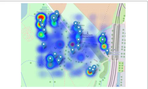
At the peak of the day, the heatmap appeared as in Fig.6. The areas appearing as "heated" in most of the cases were the toilets (top-left), the festival entrance (mid-right) and the beer stand (bottom-left).
The heavy processing was done by the Trilaterator component. Since each Trilaterator processes one set of readings and only receives a new one when it finishes there are minimum requirements from each of them. For budget efficiency a f1-micro (1 vCPU, 0.6 GB memory) instance type in Google Cloud Compute was selected. Such a machine, could do some minor filtering (clearing readings from the same access points) and trilateration, on average, in 56 ms. Considering that about 80% of the mea-surements that were sent for trilateration were unqualified mainly because they contained readings from less than 3 access points, it is obvious that an increase in the num-ber of access points would increase the processing time of each measurement from 56 ms to higher values.
In the current setup, a single Trilaterator could handle
about 1071 measurements per minute. As seen in (Fig.4),
this threshold was exceeded multiple times during the
evenings of the 21st and 22nd of July, resulting in scaling commands to be issued by the Load Balancer. The load balancing algorithm that regulated the scale in and out commands had to take into consideration the following facts:
• It takes between 25-30 s (HTTP request round trip time) to Google Cloud to create a new instance on a f1-micro machine type with an Ubuntu 16.04 image and an external IP.
• It takes almost 3.5 min (HTTP request round trip time) from the moment that the new Trilaterator is created, to connect to the Load Balancer and start consuming data. This time is attributed to the startup script for the Trilaterator, that included the
installation of "git", "node", "npm" and “forever” and the deployment and execution of the application. • It takes about 11 s (HTTP request round trip time)
for Google Cloud to stop a VM and, thus, disconnect it from the Load Balancer.
Fig. 6View of the heatmap. Heatmap at the peak of the festival according to the application
the particularities of Google Cloud. A key-concept is to allow for the same application to be used with other public cloud providers in the future with minimum intervention from the festival organizers’ side.
Based on these facts, the Load Balancing algorithm issued scaleout commands so as to ensure that each con-nected and each requested (but not yet concon-nected) Tri-lateror would be assigned 1000 measurements per minute. On the other hand, the Load Balancer was more strict with the issuing of scalein commands, which it did when the corresponding threshold was set to 200 measure-ments per minute per Trilaterator. Due to the fact that scaleins were implemented almost immediately, the algo-rithm blocked the issuing of scalein commands when there where pending scaleouts or scaleins. The latter, allowed for dealing efficiently with the case of fluctuating, yet gradually increasing loads, like in the evenings of the 3 high-traffic days without the need of prewarming the Load Balancer. On the downside, it resulted in cases where more Trilaterators than required where assigned due to the slow cooldown effect (only 1 Trilaterator is deleted at a time).
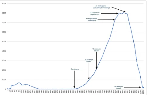
In order to provide an example of how the load bal-ancer scales, we consider a case where the load increases
rapidly (burst) within a 8 min period. Figure 7
illus-trates the fluctuation of the load balancer queue uniformly spread within 1 min intervals. It is presented this way for
producing a more readable chart. In practice the load arrives in infrequent bursts resulting in multiple scale commands to be issued at once.
We notice that the burst starts at the middle of the chart, at which point the system operates with its sin-gle, standard trilaterator. For the following 5 min the load
increases at an average rate of ∼200 measurements per
second. About 10 scaleout commands are issued almost simultaneously after 90 seconds to 100 seconds once the burst started and another 10 new trilaterators were
requested∼80 seconds later, reaching the upper threshold
of 20 spawned trilaterators operating at once. Every tri-laterator needed about 4 min to be operational since the issuing of a scaleout command. By the time that the length
of the queue reaches∼7300 objects, 10 new trilaterators,
Fig. 7Scale operations impact on load. Load balancer queue length fluctuation in an extreme case
The evaluation of the location estimation accuracy was achieved by comparing the estimations with values retrieved on the field at registered time intervals. The average haversine distance between the controlled test and the estimation was used as an evaluation metric. This test was conducted before the anonymization of the dataset, as the id (MAC address) of the control device was needed. The results showed an average declination of 10.67 meters which was marginally acceptable for the purposes of the application.
Conclusions
The main functional specifications for this application revolved around a near-real-time localization service with mediocre accuracy. The specific key performance indi-cators were set to 1 min response time and a deviation of max 12m in the location estimation. This accuracy requirement is almost 2 times the accuracy of a
smart-phone’s GPS (4.9 m according to [37] or more when
trees and other obstacles are in the area5), which can be
acceptable when other restrictions (e.g. bandwidth lim-itations, battery drainage, the need to install additional applications) hold. The conditions to which this
exper-5https://www.gps.gov/systems/gps/performance/accuracy/
imental application was tested were unique. In about
12,600 m2, part of a music festival grounds, 24
Rasp-berry Pi devices, acting as WiFi access points, collected the RSSI from an average of 318 smartphones per minute for a 3-day period. With the load becoming x8 times higher during peak times, the application should grace-fully scale to cope with the demand and continue con-suming the complete set of measurements delivered on a 1 min basis. We opted for a rather relaxed accu-racy goal in order to obfuscate the exact position of the users.
The application was implemented as a component pipeline that allowed the scaling of the Trilateration com-ponent so as to cope with the near real-time require-ments. Each component of the pipeline was implemented on Node.js and they communicated with one another through websockets. This implementation proved effi-cient and allowed the practically continuous flow of the high-frequency data streams.
of using redundant information from multiple sensor nodes.
In terms of scalability, the Google Cloud Compute resources and API proved very efficient in assisting the application scale gracefully. At the same time the appli-cation architecture itself allowed for a minimized cost, since there were limited requirements for the spawned machines. At the end, the cost of the Google Cloud infras-tructure for a complete run for the three days, plus the preceding tests, summed to roughly 80$.
Finally, it is worth noting that this experimental setup was tested under the premise that the number of atten-dants that kept their devices’ WiFi transceivers on, is ade-quately large to give an accurate perception of the overall asymmetric crowd density. The success of the experi-ment, led the festival organizers to consider increasing the number of Raspberry PI devices for the future festi-vals. The alternative of using the GPS-based localization system of the official mobile app of the festival yielded a 5% of the amount of participants recorded in comparison to STRAND. This difference shows that for one reason or another, it is not possible to acquire a critical mass of measurements for the purposes of the application.
Among the limitations that potential practitioners of this software might face, is the fragile way to estimate the distance using the signal strength. For each access point, multiple experiments must be conducted to fine-tune the formula which is something generally difficult in outdoor locations due to the potentially large number of such access points.
Availability & requirements
Project name& STRAND
Project home page & http://snf-825292.vm.okeanos. grnet.gr/ktserpes/STRAND
Operating system & Platform Independent (originally for Ubuntu Linux)
Programming language& NodeJS (Javascript)
Other requirements & NodeJS v8 or higher, Google Cloud Project
License& Apache v2.0
Restrictions to use by non-academics& License applies
Abbreviations
AP: Access point; API: Application programming interface; AoA: Angle Of arrival; DD-WRT: DresDren-wireless rouTer; HTTP: HyperText transfer protocol; MAC: Media access control; PLEX: Path loss EXponent; REST: REpresentational state transfer; RPS: Requests per second; RSSI: Received signal strength indicator; STRAND: Scalable TRilaterAtion with NoDe.js; TDoA: Time difference Of arrival; ToA: Time Of arrival; TOF: Time Of flight; VM: Virtual machine; WiFi: Wireless fidelity
Acknowledgements
The Cloud resources for the expertiment and the deployment of the software were generously provided by Google, through the GCP research credits program.
Authors’ contributions
KT is the main developer of this software. He also is the main author of this work. MP provided the background for the trilateration process. IV contributed in the system architecture when processing spatiotemporal data. All authors read and approved the final manuscript.
Funding
This work has been funded by the European Unions Horizon 2020 research and innovation programme under grant agreement no. 723131, in the frame of the joint research project “BASMATI” (http://www.basmati.cloud) and grant agreement no. 777695, in the frame of the joint research project “MASTER” (http://www.master-project-h2020.eu).
Availability of data and materials
A large subset of the original data is openly provided in Zenodo [4]. The dataset has been appropriately processed so as to make the de-identification of the users and the actual locations impossible. In particular, MAC addresses have been replaced by pseudo-IDs and the location coordinates have been shifted in a different reference point (normalized). These changes do not affect the quality of the data, nor the outcome in the case of an experiment reproduction.
Competing interests
The authors declare that they have no competing interests.
Author details
1Department of Informatics & Telematics, Omirou 9, GR17778 Tavros, Greece. 2Foundation for Research and Technology Hellas, 100 Nikolaou Plastira str,
GR70013 Heraklion, Greece.
Received: 28 November 2018 Accepted: 29 October 2019
References
1. Al Nuaimi K, Mohamed N, Al Nuaimi M, Al-Jaroodi J (2012) A survey of load balancing in cloud computing: Challenges and algorithms. In: Network Cloud Computing and Applications (NCCA), 2012 Second Symposium on. IEEE. pp 137–142.https://doi.org/10.1109/ncca.2012.29 2. Altmann J, Carlini E, Coppola M, Dazzi P, Ferrer AJ, Haile N, Jung YW, Kang
DJ, Marshall IJ, Tserpes K, et al. (Krakow) Basmati-a brokerage architecture on federated clouds for mobile applications. In: CGW 2016 International Workshop. Seoul National University, Technology Management, Economics, and Policy Program (TEMEP).https://ideas.repec.org/s/snv/ dp2009.html
3. Altmann J, Al-Athwari B, Carlini E, Coppola M, Dazzi P, Ferrer AJ, Haile N, Jung YW, Marshall J, Pages E, et al. (2017) Basmati: An architecture for managing cloud and edge resources for mobile users. In: International Conference on the Economics of Grids, Clouds, Systems, and Services. Springer. pp 56–66.https://doi.org/10.1007/978-3-319-68066-8_5 4. Altmann J, Aryal RG, Carlini E, Cho C, Coppola M, Dazzi P, Haile N, Jung
YW, Karaboga B, Kim SW, Kim M, Koo WB, Lechler C, Lopez L, Marshall IJ, Marshall CLT, Marshall K, Pages E, Psomakelis E, Santoso GZ,
Schwichtenberg A, Sok SW, Tserpes K, Varvarigou T, Violos I, Wacker R, Zylowski T (2019) Basmati wifi localization.https://doi.org/10.5281/ zenodo.3333032
5. Bas E, Tekalp AM, Salman FS (2007) Automatic vehicle counting from video for traffic flow analysis. In: 2007 IEEE Intelligent Vehicles Symposium. IEEE. pp 392–397.https://doi.org/10.1109/ivs.2007.4290146 6. Boominathan L, Kruthiventi SS, Babu RV (2016) Crowdnet: A deep
convolutional network for dense crowd counting. In: Proceedings of the 24th ACM international conference on Multimedia. ACM. pp 640–644. https://doi.org/10.1145/2964284.2967300
7. Boonsriwai S, Apavatjrut A (2013) Indoor WIFI localization on mobile devices. In: 2013 10th International Conference on Electrical Engineering/Electronics, Computer, Telecommunications and Information Technology. pp 1–5.https://doi.org/10.1109/ECTICon.2013. 6559592
8. Chauhan A (2015) Systems and methods for providing load balancing as a service. Google Patents. US Patent App. 14/282,411
survey. Comput Netw 110:284–305.https://doi.org/10.1016/j.comnet. 2016.10.006
10. Di Domenico S, De Sanctis M, Cianca E, Colucci P, Bianchi G (2017) Lte-based passive device-free crowd density estimation. In: 2017 IEEE International Conference on Communications (ICC). IEEE. pp 1–6.https:// doi.org/10.1109/icc.2017.7997194
11. Fang Y, Wang F, Ge J (2010) A task scheduling algorithm based on load balancing in cloud computing. In: International Conference on Web Information Systems and Mining. Springer, Lecture Notes in Computer Science, vol 6318. Springer, Berlin, Heidelberg. pp 271–277
12. Gavin H (2011) The levenberg-marquardt method for nonlinear least squares curve-fitting problems. Department of Civil and Environmental Engineering, Duke University
13. Gharghan SK, Nordin R, Ismail M, Ali JA (2016) Accurate wireless sensor localization technique based on hybrid pso-ann algorithm for indoor and outdoor track cycling. IEEE Sensors J 16(2):529–541
14. Gupta G, Bhope V, Singh J, Harish A (2018) Device-free crowd count estimation using passive uhf rfid technology. IEEE J Radio Freq Identif 3(1):3–13
15. Hu J, Gu J, Sun G, Zhao T (2010) A scheduling strategy on load balancing of virtual machine resources in cloud computing environment. In: Parallel Architectures, Algorithms and Programming (PAAP), 2010 Third International Symposium on. IEEE. pp 89–96
16. Lanzisera S, Zats D, Pister KS (2011) Radio frequency time-of-flight distance measurement for low-cost wireless sensor localization. IEEE Sensors J 11(3):837–845
17. Leinberger W, Karypis G, Kumar V, Biswas R (2000) Load balancing across near-homogeneous multi-resource servers. In: Heterogeneous Computing Workshop, 2000. (HCW) 2000 Proceedings. 9th. IEEE. pp 60–71.https://doi.org/10.21236/ada439559
18. Li Z, Braun T, Dimitrova DC (2015) A passive WiFi source localization system based on fine-grained power-based trilateration. In: 2015 IEEE 16th International Symposium on A World of Wireless, Mobile and Multimedia Networks (WoWMoM). pp 1–9.https://doi.org/10.1109/ WoWMoM.2015.7158147
19. Lu Y, Xie Q, Kliot G, Geller A, Larus JR, Greenberg A (2011) Join-idle-queue: A novel load balancing algorithm for dynamically scalable web services. Perform Eval 68(11):1056–1071
20. Makris A, Tserpes K, Andronikou V, Anagnostopoulos D (2016) A classification of nosql data stores based on key design characteristics. Procedia Comput Sci 97:94–103.https://doi.org/10.1016/j.procs.2016.08. 284. 2nd International Conference on Cloud Forward: From Distributed to Complete Computing
21. Makris A, Tserpes K, Anagnostopoulos D, Altmann J (2017) Load balancing for minimizing the average response time of get operations in distributed key-value stores. In: Networking, Sensing and Control (ICNSC), 2017 IEEE 14th International Conference on. IEEE. pp 263–269
22. Mishra SK, Sahoo B, Parida PP (2018) Load balancing in cloud computing: A big picture. J King Saud Univ - Comput Inf Sci.https://doi.org/10.1016/j. jksuci.2018.01.003.http://www.sciencedirect.com/science/article/pii/ S1319157817303361
23. Mitilineos SA, Kyriazanos DM, Segou OE, Goufas JN, Thomopoulos SC (2010) Indoor localisation with wireless sensor networks. Progress In Electromagn Res 109:441–474
24. Oguejiofor O, Aniedu A, Ejiofor H, Okolibe A (2013a) Trilateration based localization algorithm for wireless sensor network. Int J Sci Mod Eng (IJISME) 1(10):2319–6386
25. Oguejiofor O, Okorogu V, Adewale A, Osuesu B (2013b) Outdoor localization system using rssi measurement of wireless sensor network. Int J Innov Technol Exploring Eng 2(2):1–6
26. Pedro D, Tomic S, Bernardo L, Beko M, Oliveira R, Dinis R, Pinto P (2018) Localization of static remote devices using smartphones. In: 2018 IEEE 87th Vehicular Technology Conference (VTC Spring). IEEE. pp 1–5.https:// doi.org/10.1109/vtcspring.2018.8417726
27. Rahman M, Iqbal S, Gao J (2014) Load balancer as a service in cloud computing. In: 2014 IEEE 8th international symposium on service oriented system engineering (SOSE). IEEE. pp 204–211.https://doi.org/10. 1109/sose.2014.31
28. Ren X, Lin R, Zou H (2011) A dynamic load balancing strategy for cloud computing platform based on exponential smoothing forecast. In: Cloud Computing and Intelligence Systems (CCIS), 2011 IEEE International
Conference on. IEEE. pp 220–224.https://doi.org/10.1109/ccis.2011. 6045063
29. Rusli ME, Ali M, Jamil N, Din MM (2016) An improved indoor positioning algorithm based on rssi-trilateration technique for internet of things (iot). In: Computer and Communication Engineering (ICCCE), 2016
International Conference on. IEEE. pp 72–77.https://doi.org/10.1109/ iccce.2016.28
30. Shen H, Ding Z, Dasgupta S, Zhao C (2014) Multiple source localization in wireless sensor networks based on time of arrival measurement. IEEE Trans Signal Proc 62(8):1938–1949
31. Siddiqui MH, Khalid MR (2012) A Robust Scheme for Tracking of a Mobile Node using WiFi Signals. Wirel Commun 4(11):609–614.http:// ciitresearch.org/dl/index.php/wc/article/view/WC072012005 32. Sindagi VA, Patel VM (2018) A survey of recent advances in cnn-based
single image crowd counting and density estimation. Pattern Recogn Lett 107:3–16
33. Spinner S, Kounev S, Zhu X, Lu L, Uysal M, Holler A, Griffith R (2014) Runtime vertical scaling of virtualized applications via online model estimation. In: Self-Adaptive and Self-Organizing Systems (SASO), 2014 IEEE Eighth International Conference on. IEEE. pp 157–166.https://doi. org/10.1109/saso.2014.29
34. Stoyanova T, Kerasiotis F, Papadopoulos G (2015) Rss-based outdoor localization with wireless sensor networks in practice. In: Technological Breakthroughs in Modern Wireless Sensor Applications, IGI Global. pp 225–256.https://doi.org/10.4018/978-1-4666-8251-1.ch010 35. Tomic S, Beko M, Dinis R (2015) Rss-based localization in wireless sensor
networks using convex relaxation: Noncooperative and cooperative schemes. IEEE Trans Veh Technol 64(5):2037–2050
36. Tserpes K (2019) stream-msa: A microservices’ methodology for the creation of short, fast-paced, stream processing pipelines. ICT Express 5(2):146–149.https://doi.org/10.1016/j.icte.2019.04.001.http://www. sciencedirect.com/science/article/pii/S2405959519301092. Accessed 29 Apr 2019
37. Van Diggelen F, Enge P (2015) The worlds first gps mooc and worldwide laboratory using smartphones. In: Proceedings of the 28th international technical meeting of the satellite division of the institute of navigation (ION GNSS+ 2015). ION GNSS+. pp 361–369.https://www.ion.org/ publications/abstract.cfm?articleID=13079
38. Wang J, Luo J, Pan SJ, Sun A (2018) Learning-based outdoor localization exploiting crowd-labeled wifi hotspots. IEEE Trans Mob Comput 39. Wang Y, Ho K (2015) An asymptotically efficient estimator in closed-form
for 3-d aoa localization using a sensor network. IEEE Trans Wirel Commun 14(12):6524–6535
40. Weppner J, Bischke B, Lukowicz P (2016) Monitoring crowd condition in public spaces by tracking mobile consumer devices with wifi interface. In: Proceedings of the 2016 ACM International Joint Conference on Pervasive and Ubiquitous Computing: Adjunct. ACM. pp 1363–1371. https://doi.org/10.1145/2968219.2968414
41. Xiong F, Shi X, Yeung DY (2017) Spatiotemporal modeling for crowd counting in videos. In: Proceedings of the IEEE International Conference on Computer Vision. pp 5151–5159.https://doi.org/10.1109/iccv.2017.551 42. Xiong H, Chen Z, An W, Yang B (2015) Robust tdoa localization algorithm
for asynchronous wireless sensor networks. Int J Distrib Sensor Netw 11(5):598,747
43. Zafari F, Gkelias A, Leung KK (2017) A survey of indoor localization systems and technologies. CoRR:abs/1709.01015.http://arxiv.org/abs/1709.01015
Publisher’s Note