Modelling Learning as Modelling
Scott Moss and Bruce Edmonds
Centre for Policy Modelling,
Manchester Metropolitan University.
Abstract
Economists tend to represent learning as a procedure for estimating the parameters of the “correct” econometric model. We extend this approach by assuming that agents specify as well as estimate models. Learning thus takes the form of a dynamic process of developing models using an internal language of representation where expectations are formed by forecasting with the best current model. This introduces a distinction between the form and content of the internal models which is particularly relevant for boundedly rational agents.
We propose a framework for such model development which use a combination of measures: the error with respect to past data, the complexity of the model, the cost of finding the model and a measure of the model’s specificity The agent has to make various trade-offs between them. A utility learning agent is given as an example.
1
Motivation
The rational expectations, consistent expectations, least-squares learning and similar hypotheses of mainstream economics are predicated on the presumption that the underlying structure of the economic environment is stable. Only on this assumption can agents who believe that they know the “correct” structural model of their environment use that model to form unbiased expectations.
Where structural change itself is an issue, this must be reflected in continual updates of the underlying formulation of agent’s models in order to reduce their forecasting bias. Indeed, one likely reason for agents to change their forecasting models is the presence of systematic bias in their forecasts.
In this paper, we describe a framework to study how agents might reduce their forecasting bias by changing the structural forms of their respective models of their environments. That is, we model economic agents as model-building forecasters rather than simply model-using forecasters who know only a given structural model.
The models our agents specify result from their observations of data and the success with which their models forecast variables of interest to them. In an environment in which there is no structural change, it also seems reasonable to suppose that, once an unbiased model with tolerable precision has been found, the process by which agents develop their forecasting models is not especially interesting. There are, however, cases in which agents’ forecasts are biased or imprecise to such a degree that they would reasonably seek to improve their models.
1. Moss acknowledges financial support from the Nuffield Foundation and from the Engineering and Physical Sciences Research Council under grant IED/4/1/8022. We also acknowledge the support of
In ef fect, agents (like economists) might devote resources to the improvement of their forecasting models. Such improvements in forecasting capabilities would be especially important during times of structural change as, for example, in emer ging market economies, where there is technological change, or perhaps at the turning point of a trade cycle.
Thus the models of learning we propose below should be particularly applicable to situations of structural change, where by “structural change” we mean that it is not merely a case of changing the parameters of the “correct” model but also changing the form of that model. A second reason for using the type of model described below , is that the agent models are meaningful. You can trace the reasons that an agent develops a particular model and hence takes a particular action. In traditional terms this is a simulation model rather than a black-box model. This is important if your primary aim is to examine and understand a process, as opposed to calculating a prediction of a future state.
In order to avoid necessary confusion we will refer to our model of how agents learn as
simply models and the models built by the agents themselves as agent models or, when the agent context is clear, internal models.
2
Criteria for a Good Model of Agent Learning
A good model is, trivially , one that meets the needs of the model users. This is true whether we are talking about an agent model or our model of an environment including such agents.
The function of economic models, for example, is often to demonstrate suf ficient conditions for the existence of equilibrium. The introduction of learning schemes into such models is often intended to demonstrate sufficient conditions under which learning makes equilibrium models stable. A classic of this genre is Bray and Savin [3], but see also Binmore and Samuelson [2], Marimon, McGrattan and Sargent [13] and Arifovic [1].
We are not concerned in this paper with equilibrium per se though we are concerned with computer-based simulation models. Such models can be used to generate point or interval forecasts or, alternatively, controlled variations on a single model structure to generate “what-if” analyses of particular business or economic policies.
2.1 Rigour
Whatever the uses to which they are put, we take the view that simulation models should not be less rigorous than analytic models. Rigour provides a set of rules according to which developments and meaning of the models can be assessed. In effect, models provide the basis for a discourse about as-yet-unrealized outcomes and, to be useful, we believe that such discourse must also be disciplined.
2.2 Incrementality of the Learning Process
One aspect of learning that seems clear is that agents frequently do not perform exhaustive searches for the best internal model of something, but adapt existing models. A good example of how well this works as a representation of actual agent model-building is Lenat’ s [12] model of how mathematicians form conjectures in number theory. This may be formalised by putting a cost on the search for new models. Even though the cost of each search step may be low, the total cost can still be signif icant. Thus discarding a model and starting again can be very costly due to the lar ge search space of possible models. In such circumstances, it is important to be able to improve models by means of a focused search in the space of possible models. This seems to us to be an appropriate policy to follow in model-building of all kinds. We therefore assume that such a policy will be followed by agents in the development of their internal models.
2.3 Examinability of models learnt by the agents
Agent models should be examinable, in the sense that the state of an agent's learning should be open to common-sense interpretation. If this is not the case then we would be able to analyse only the agent's behaviour rather than the process by which it was generated. While this may be realistic for the modelling of agents who model other agents, this is unhelpful from our point of view as modellers seeking to understand the ef fects of specific approaches to agent learning and expectations formation. The internal states of the agents can be made opaque to other agents without sacrif icing our knowledge of those states. Furthermore, if we can choose the extent to which an agent is aware of the internal states of other agents, then we can model and contrast this aspect as well.
2.4 The existence of different trade-offs in model search
The most useful model for an agent would be one which, with complete conf idence, gave point forecasts of every tar get variable for every feasible set of values of the decision variables and yet was reasonably simple. The purpose of model adaptation is to move from the default position towards the best position. This involves the best possible increase in precision with the least possible complexity . A noble sentiment completely without operational content and one which is, of course, not always possible. The guides to model improvement, should be able to include:
The error (e.g. RMSE) of the model’s predictions. Clearly, a model with less error is better.
• The complexity of the model. A simpler model is better than a more complex one for an The cost of searching for a model.
• The volume, a summary measure of precision and generality, described below.
with distinctly limited resources (a start-up?) looking for an opportunity in a fast moving environment might settle for a less accurate and vaguer model.
2.5 The importance of the form of the agent’s models
The agent will have some language to represent its models. In fact, it can only represent its models by expressions in this language. This creates a mapping between expressions in the language and subspaces of possibilities, that corresponds to the distinction between the syntax and semantics of a logical language. In AI parlance this is called a Logical Bias. This fact has several consequences, including these listed below.
• Only some subspaces will be expressible in the language, the agent may be forced to approximate the actual subspace of possibilities with an expressible one.
• Some subspaces will have several corresponding expressions, some of which will be far more efficient to use than others.
• Although the agent will often know what the space of possibilities in some theoretical sense, she will often not know what expressions are necessary to describe a particular subspace, thus for all practical purposes the space of possibilities is unknown and unknowable.
• A global search of possible subspaces is impractical, because the agent has to do this by searching through possible expressions in her language. This involves a dif ferent kind of search than that of paramaterising a known agent model.
• If there is any significant cost associated with building the agent model expressions then some sort of incremental, path-dependent development of agent models is inevitable.
• The agent may come to believe in inadequate or even partially inconsistent expressions. These would be less likely to be successful models, but are not automatically ruled out (depending on the agent language).
2.6 Expressiveness of the Internal Language of Representation
In order that the agent’s may be able to change the form as well as the parameterisation of its models of its world, the agent needs to be equipped with a language with which to do this. Such a language will have a syntax in the sense of a grammar which determines the sort of expressions that are allowed as candidate internal models. It will also have a semantics in the sense of some correspondence between these expressions and their referents in the agent’ s environment.
2.7 Practical to simulate
In order that this representation be a practical research tool it is necessary that there is some reasonably ef ficient decision procedure that successfully implements the agents’ modelling process.
3
Alternative learning paradigms
T
able
1:
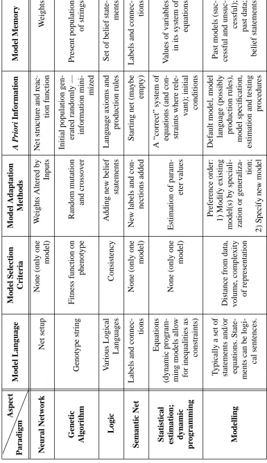
A Comparison of Learning Paradigms
Model Language Model Selection Criteria Model Adaptation Methods A Priori Information Model Memory Neural Network Net setup
None (only one
model)
W
eights Altered by
Inputs tion function W eights Genetic Algorithm Genotype string
Fitness function on
phenotype
Random mutation
and crossover
Initial population
gen-erated randomly — information
mini-mized Present population of strings Logic V arious Logical Languages Consistency
Adding new belief
statements
Language axioms and
production rules
Set of belief
state-ments
Semantic Net
Labels and
connec-tions
None (only one
model)
New labels and
con-nections added
Starting net (maybe
empty)
Labels and
connec-tions
Statistical estimation; dynamic
pr
ogramming
Equations
(dynamic program- ming models allow for inequalities as
constraints)
None (only one
model)
Estimation of
param-eter values
A “correct” system of equations (and
con-straints where
rele-vant); initial conditions
V
alues of variables in its system of
equations
Modelling
T
ypically a set of
statements and/or equations. State- ments can be
logi-cal sentences.
Distance from data, volume, complexity
of representation
Preference order:
1) Modify existing
model(s) by speciali- zation or
generaliza-tion;
Default model, model
language (possibly production rules),
model specification,
estimation and testing
procedures
Past models (suc- cessful and unsuc-cessful); past data;
belief statements
Paradigm
The two particular aspects of these models which are of greatest interest here are the model selection criteria and the model adaptation methods. On the criterion of model selection methods alone, network representations of learning and learning as statistical estimation differ fundamentally from the modelling representation and genetic algorithms in that there is only one model and, so, no selection to be made. On the criterion of model adaptation methods, modelling has most in common with neural networks and logics in relation to model specification and shares with rational expectations and least-squares learning a reliance on the estimation of model parameters.
Genetic algorithms and evolutionary methods engage in some sort of random search which generates new models which are selected with increasing frequency if they do well and with less frequency until they are discarded if they do badly . Genetic algorithms become increasingly local in their model adaptations as they identify the areas of the model space which systematically yield the fittest models.There is a single process by means of which genetic algorithms identify the best models and the estimate the best values of the parameters of those models.
The closeness among modelling, neural networks, genetic algorithms and logics in model specification is that all of them modify the hypothesized relationships among variables by marginal changes resulting from specific failures of the incumbent models.
In summary, the modelling representation of learning differs from all of the others but logics and genetic algorithms in allowing for multiple models and for adapting models only by local searches of the space of possible models.
Some logics can be used to represent learning as modelling. Several of these have been devised and implemented ( e.g., Masuch and Huang [15]; Fox, Krause and Elvang Goransson [9]. Others (e.g. Fagin and Halpern [10]; Fox [8]) have been well explored.
It seems reasonable to require a representation of learning as modelling to be sound and consistent. In general, completeness and decidability are desirable for the (real, i.e. not simulated) model-builder but only be obtainable at the expense of the expressive power of the formal framework.
This is in contrast to the situation with the internal models of the agent. Here the logic paradigm has more problems, principally logical omniscience, and the common tolerance of inconsistency. There are logic formalism which get round these problems (for example step logics and paraconsistent logics), but still do not map naturally into learning as it is preformed by real economic agents.
4
Agent Models with defaults
Our criteria for a good agent model suggest that any representation should clearly specify the dependent variables, the independent variables, the expression specifying the relationship between them and the conditions of application of the model.
Each of these should have a default value. T aken together, these default values ef fectively define some a priori information available to agents. They might know , for example, which are their decision variables and which are their goals. They might believe there is some relationship between them without knowing either what that relationship is or in what conditions any such relationship might hold. More precise default values will indicate more a
priori knowledge held by agents. This a priori information may be implicitly encoded in the
model structure described below in a natural way by the specification of the language in which the agent develops its models.
In many cases, the default value of the dependent-variables will be the set of tar get variables defined in the model of the environment and the default value of the independent-variables will be all of the decision-variables which the environment allows individual agents. The relationship will say that for any value or set of values of the decision variables, the tar get variables can take any (set of) feasible values. If, for example, the tar get is profit and the decision variable is price, then the initial (default) position is that for any feasible (i.e. non-negative) price, profit can take any rational value. The conditions of application will have by default a value indicating complete generality . Typically, this will be indicated by the simple value true since the conditions of application are either satisfied or not and, collectively, should return a boolean value.
The agents will, in general, have other a priori knowledge, including:
1. knowledge implicit in the grammar of its internal modelling language mentioned above; 2. maybe some explicit knowledge encoded as an initial model given to the agent (e.g.
accounting rules);
3. knowledge encoded in a basic algorithm for learning (improving its models); and some goals.
5
Criteria an agent might use in the search for a good internal
model.
The following sub-criteria should inform actual and agent searches for “better” models.
5.1 Accuracy
This is the straightforward notion that a good model will yield forecasts which are unbiased and efficient. We would not, however, expect all good models to yield accurate forecasts in all circumstances. The economic and methodological reasons for this were discussed by
5.2 Measures of Model Specificity
5.2.1 Generality
The generality of a model is def ined by the conditions in which it is applicable. A model is made unambiguously more general by subtracting from the set of its conditions of application. It is made less general (or more specialized) by adding to the set of its conditions of
application.
For example, if a model is found sometimes to forecast accurately and other times to forecast inaccurately, the natural procedure is to determine the special conditions in which the model is a useful guide to action. A natural presumption is that additional conditions of application are required. This will require some procedure to discriminate amongst those additional conditions for which the model holds and those in which it does not hold. If such a procedure is successful, a better model will result which dif fers from its forebear in having a lar ger number of conditions of application. It will therefore be applied in a more restricted set of cases.
5.2.2 Scope
We take the scope of a model to be the Cartesian product of all possible values of its
dependent and independent variables. The scope of a model is increased by adding to (and is reduced by subtracting from) the set of variables over which it is defined. Increasing the scope of a model can vastly increase the specif ic forms that the model takes. In general, increasing model scope is to be avoided if at all possible because it necessarily increases the
computational and information-processing capacities that the model will absorb. One of the advantages of generalizing models is that the generalized model may have fewer independent variables than the models it replaces and, so, a smaller scope.
5.2.3 Precision
The precision of a model is the range of the dependent variables of the model corresponding to any point in the domain of the independent variables. An example will indicate the importance of the precision of the model. High pressure weather systems are
thermodynamically more stable than systems dominated by low pressure. Consequently , the precision of forecast movements and ef fects of high pressure systems is greater than the precision of forecasts of weather systems dominated by low pressure. Interval rather than point forecasts may often be appropriate. However , adaptations of the model to reduce the range of the interval — that is, to increase the precision of the model
5.2.4 Volume
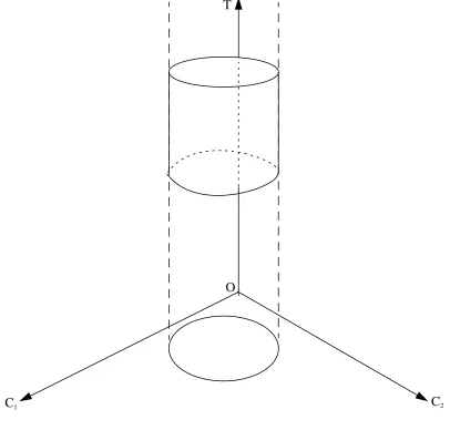
In this paper we will summarise scope, precision and generality into a single measure which we will call the volume of the model. The volume of the default model suggested in section 4 is the volume of the feasible part of the space of decision and tar get variables. The model volume can be reduced by special models which exclude parts of that space. The volume of a model is a rough measure of its refutability (as in Popper [22]), the ease with which it could be disconfirmed (if its wrong).
mapping from control variables C1 and C2 into the target variable T. The domain of the relation
is the ellipse in the plane C1OC2. The height of the cylinder is the precision of the model. That
is, given any pair of values of C1 and C2, say and ,the value of T will be determined by
some point within the cylinder on a line perpendicular to the C1OC2plane at ( , ). The
relation does not indicate which point on that line will yield the realized value of T. Since this is true for any point within the cylinder, the size of the collection of such points is the volume of the cylinder. Since the cylinder is the mapping between the independent and the dependent variables, its volume is naturally identified with the volume of the relation.
We shall say that the agent has a universal model which comprises the whole of the
C1,C2,T)-space except in the domain of the cylinder . It will be in keeping with natural use of
language if we call the cylinder a special model for the domain represented by the ellipse in the C1OC2-plane. The default values continue to apply everywhere else in ( C1,C2,T)-space.
The volume of the universal model is now the volume of the feasible space minus the volume of that space which is in the domain of the cylindrical model plus the volume of that model (the volume of the cylinder). In other words, the volume of the agent’ s universal model is
Figure 1: : Domain, Range, Precision and Volume.
Cˆ1 Cˆ2
Cˆ1 Cˆ2
C1 C2
T
reduced by the volume of the space above and below the cylindrical special model. Clearly , the volume of the universal model can be reduced further either by increasing either the domain of the cylindrical model or its precision. Moreover , special models with dif ferent domains from that of the cylindrical model will also reduce the volume of the universal model. So, too, will models of lesser dimension than the whole of the ( C1,C2,T)-space. If a
relationship between (say) C1 and T can be found over some domain of C1 and some range of T, then in ( C1,C2,T)-space the special model is a bar , rectangular in cross-section projected
perpendicularly from the rectangle in the C1OT plane implied by the domain and range of the
two-dimensional model. The volume of the universal model is therefore reduced by the volumes above and below that bar in the feasible space.
The perfect model has perfect precision and, therefore, zero volume in space of any dimension — just as a point, a line or a plane have zero volume in three dimensions. The volume of the least restrictive model is the volume of the feasible part of a space with dimensionality equal to the number of all of the variables which define the state of the environment. Reducing the dimensionality of the model, increasing the domain of the special models and/or increasing the precision of special models all reduce the volume of the agent’s universal model. We take reduction in model volume to be a criterion of improvement and, therefore, a guide to model adaptation.
The default assumption is that anything is possible. Only those possibilities within the domain of the model description that are not predicted by that description are ruled out. So if the domain of applicability of the model description is narrowed (by, say, adding extra conditions) then fewer possibilities will be ruled out - the total volume increases. If the precision of the prediction of the model description is increased, then within this domain more possibilities are ruled out - the total volume decreases. Thus by these definitions, condition 3 above implies that models which give more precise predictions and those with wider conditions of application are preferable. Also models with a smaller volume are more easily falsifiable, in the sense that a random possibility is more likely to lie outside the volume of possibilities predicted by the model and thus show it to be wrong.
5.3 Cost
In a purely numerical modelling language, the semantics is a one-one correspondence, so the distinction between the form of the model (a set of parameters) and what they refer to (a set of quantities) can be identif ied with each other without confusion. Given the more expressive language as illustrated immediately above, this correspondence will be more complicated. For example there may be several different expressions that refer to the same set of relations in the agent’s environment, but one of these may be much more ef ficient to use for prediction than the other. This is important for agents with limited rationality. Thus the form of models as well as the content become important.
5.4 Complexity
One way to bias the agent towards agent models that are more likely to be productive is to limit its agent modelling language to rule out models comprising nothing more than past observations. This, however, would probably mean a more restricted language than is sometimes desirable and would probably not rule out all analogous situations within the new language.
A second way is to include some element of complexity to guide model search, i.e. in certain circumstances (e.g. when error rates are almost equal) bias the agent to choose the simpler model. We are not claiming that the simpler model is a priori more likely to be correct (Quine [23], Pearl [21]), just that this is an ef fective heuristic for search within such open-ended spaces of language expressions.
There are many possible ways to measure complexity (Edmonds [6]) and each will result in a slightly different search pattern. All we require is that the measure be practically computable and that it can act as a limit to naive depth-first strategies that might be applied by an agent.
6
Some Possible Agent Strategies
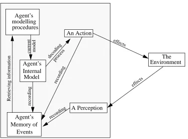
The difficult aspect of modelling learning as modelling is to represent the ways in which the agent adapts its model based on the actions it has taken and the input it has received. In this section, we describe one possible representation of the information f lows involved. A legitimate and important issue is surely the choice or development of the representation of the agent modelling procedure.
If we are looking at abstract environments with no direct, empirical referent, then the purpose of the representation of the modelling procedure is to show that a particular learning procedure will generate results which an agent would find desirable or , alternatively, that in the simulated environment, some modelling procedures are likely to yield better values of target variables than other learning procedures. This sort of result is not obviously less relevant or important than the standard economic procedure of demonstrating suf ficient but not necessary conditions for the existence of equilibrium.
An alternative use of the learning-as-modelling paradigm is to represent aspects of actual economic environments. In these cases, the measure of the goodness of the learning representation is the extent to which the simulation models generate output which conforms statistically or qualitatively to observed outcomes. W e recognize that these ar guments will carry no weight with those for whom there is no economics without equilibrium. But the developments reported here will, in any case, be of little relevance to such economists.
goals on the other. These relations evolve as changes in weights attaching to network links in the case of neural networks. Where production systems and logics are concerned, the relations of which a model is comprised can be mnemonic and explicit. Simple models can be built up into more complex models. The way in which model complexity increases can itself become a subject of study.
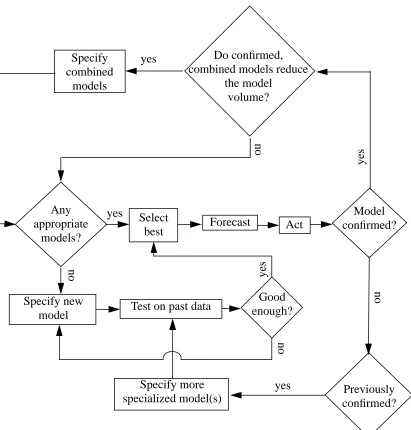
In figure 3, we depict the flow chart of an algorithm which lends itself readily to implementation as a production system. The natural starting point in this flow chart is the question: Any appropriate models? Initially, there would be no model other than the universal or some default model. By definition, only special models can be appropriate bases for action
Figure 2: : Information flows in learning procedures
Agent’s modelling procedures
Agent’s Internal Model
An Action
A Perception Agent’s
Memory of Events
The Environment
recording
recording current model
effects
effects decoding
process
recording
since, without a relevant special model the universal model says only that anything can happen..
A model is appropriate if it has conditions of application that are satisfied in the current state of the environment. If there is no appropriate model in this sense, then there must be some means of conjecturing new models. Typically, such conjectures will be formulated or, at least, tested on the basis of past data. Respecification and re-estimation may continue until there is some model which is deemed to be “good enough” in the circumstances or , simply, the modeller decides that no more resources are to be devoted to the development of an appropriate model. If there is already at least one model with satisfied conditions of application, then there is no need at this stage to specify additional models. In either case, choose a model which is “best” according to some set of criteria.
Figure 3: A Possible Learning Algorithm
Any appropriate
models?
Select best
Specify new
model Test on past data
Good enough?
Forecast Act confirmed?Model
Previously confirmed? Specify more
specialized model(s)
Do confirmed, combined models reduce
the model volume?
yes
yes
yes
yes Specify
combined models
yes
no
no
no
It would be natural to use the “best” of the appropriate models to forecast the effects on goals of different values of the decision variables and, on the basis of such forecasts, to set the decision variable value which, in this context, is what we mean by an action.
The next question is whether the action had the intended ef fect. If not, the model is disconfirmed. But it might be that the same model had previously been used successfully to determine an action. In that case, it would be appropriate to try to distinguish the conditions in which the model succeeded from those in which it failed. This will involve some attempt to specialize the model by adding conditions of application. The resulting specialized model is then subject to the same tests as any other newly specified model.
A model which serves successfully as a guide to action might, in combination with other successful models, be generalizable. One possibility is to see if there is a meaningful intersection in their respective conditions of application as well as some suitable way of combining their definitions, independent and dependent variables. In this way, we would have one model which was applicable in a wider set of conditions with a domain and range no less than that of the constituent models taken together . As indicated in the flow chart in figure 3, combinations of special model should have the effect of reducing the volume of the universal model if they are to be desirable.
6.1 Example strategies for agent model development
6.1.1 Crossover
In genetic programming (Koza [11]) the principle operation for model development is crossover . This is where random points in two models are selected and the appropriate submodels are swapped. This is a highly ef fective operator which has been used in solving many real-life problems. Its advantages are its speed, the fact it is universal in the sense that sequences of crossover operations can be used to construct any model (from a suitably lar ge initial population), it preserves the variation in the population as well as the average depth of the population. From a perspective of modelling learning however , it is inappropriate due to its arbitrary action, the globality of its search and its need for very large populations of models to act upon.
An agent model can be effectively defined as a data structure with four slots: the independent variables, the dependent variables, the relationship between them and the conditions of application. Any adaptation of an agent model entails changes in the values of these slots. In this section we discuss coherent model-adaptation strategies in relation to the generalization and specialization of the agent’s special models.
6.1.2 Specializing the agent’s model.
Specialization of a model always increases the volume of the universal model and, so, is to be avoided where possible. Adding conditions of application always specializes an existing model. So, too, does increasing the scope of the model by adding variables. Anything which reduces the domain of a special model is obviously a specialization. It seems sensible to recognize any volume-increasing adaptation of a model as a specialization.
When an agent adds a new variable to his model, this does not change the space of possibilities but it does change the size and perhaps the complexity of the model description. When the new variable is defined in terms of existing variables, it is a purely formal device in the model description, as whenever it occurs, the original reference to the variables it was defined by could be substituted instead. Placing conditions on this new variable is equivalent to a restrictive condition on the possible combinations of the environmental variables.
Take an example where there are two input variables v and w and one output variable p. If there is an existing model of the form p=g(x,y) for some relation g then the agent might try a model of the form p=f(v) where using some a priori information about the
dimensionality of variables. The agent has thus decomposed the model into two separate parts to reduce the information considered. In effect, new conditions are added by specifying some relationship between the outputs of the models and combinations of the inputs to the model. This is a clear specialization of the original model (It is also an unambiguous simplification of the model as will be seen in section 7).
Model specialization takes the following form:
1. Combine existing variables into a new variable in such a way that the number of dimen-sions of the new variable is less than the number of dimendimen-sions of the component variables. The only exception is combinations of pure numbers which are themselves pure numbers. 2. Assess whether the changes in or values of the new variable discriminate between cases in
which any model is disconfirmed and cases in which it is not.
3. If it is found to have some discriminatory power , specialize the model by adding the appropriate statement to its conditions.
6.1.3 Generalizing models of the agent.
This would be tried when the agent has two models which are well conf irmed according to some criterion. Generalization entails taking the intersection of the antecedents and the union of the consequents of the two models as the elements of the antecedents and consequents of the new model. The new model would apply in a wider range of conditions including at least all of the conditions in which both of the models from which it is generalized would apply . It would also forecast the values of a wider range of variables.
Generalizations will not be accepted if the resulting set of consequent clauses are either contradictory or cannot be instantiated from the resulting set of antecedent clauses. One implication of this condition is that the antecedents cannot be empty unless all of the values set by the generalized consequent are constants.
7
Towards a Specification of a Framework for Modelling
Economic Learning by Modelling
There will not be a complete logical formalism of the described learning mechanism, as it is not necessarily deterministic in nature. However some aspects can be so captured, particularly the relationship at any one time between an agent’s models and the environment.
7.1 The General Framework
7.1.1 The Space of Possibilities
There is a space of possibilities, PS, inherent in the agent’ s environment. T ypically in simulations this space will usually be a product of a limited number of spaces,
representing the different variables (one of which may be time). In many economic simulations these spaces, , will just be either boolean or a finite range of numerical values, for example a range of prices of limited range and precision. More
generally these spaces could themselves be a space of language expressions, for example, a language of negotiation. If the language includes binary relations onV, for example expressing that today’s price is always at least as great as yesterday’s, then the space of possibilities may need to be , and lar ger for tenary relations (etc.). Of these spaces, , typically some will be decidable by the agents (settable by its action), some will be directly observable and others will only be indirectly inferrable.
7.1.2 The Internal Language of Representation.
The agent has an internal language of representation, L, which is recursive list of expressions, . Usually L will typically be def inable as nothing stronger than a context free grammar based on a f inite list of atomic symbols. In this case they would correspond to tree structures.
Each expression specifying an internal agent model will include the dependent and independent variables, its conditions of application, the default prediction when conditions fall outside this, in addition to the relation between the variables. T ypically much of this information is specified implicitly through the nature of L, the mechanisms to infer a prediction or action and common defaults.
7.1.3 The semantics of L
There will be a mapping ,which will reflect the natural semantics of L in the space of possibilities,PS. Each member,l, ofL refers to a subspace, m(l) (this, after all, is the point of such models). This mapping is usually not a 1-1 mapping, in that not every possible subspace ofPS is mapped to by a member ofL.
As discussed in section 2.5 this allows for the possibility of genuine surprise, when the agent faces some behaviour of its environment which it could not model. It is maybe this syntactic/semantic split that most dif ferentiates this approach from a more traditional economic approach, where is sometimes assumed that behaviour of the economy and the model the agent uses are basically the same.
In general allowed models of L, will be only those that are consistent with the given a piori knowledge that the agent has, i.e. those which refer to subspaces of the space referred to by this knowledge. It is usual for the syntax of L, to be designed so that all expressions in L
correspond to allowable models.
V = v1 v2 … vn
v1, , ,v2 … vn
PS = V2 v1, , ,v2 … vn
l1, ,l2 …
{ }
The indicators for the agent (utility , pain, profit etc.), are functions of the actual resulting position in PS, from which the agents goals may either be specified (or even inferred by the agent). This goal also corresponds to a subspace ofPS.
Finally the agents knowledge of past behaviour can be represented by a series of data points in
PS.
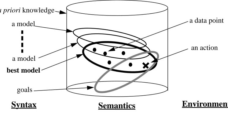
The general structure is illustrated in figure 4
7.2 A specification of the agent
Thus at any time,t, an agent has:
1. a set of models: , from which it will have to select the model it will use
for deciding its action and which it base future models on;
2. memory of past data: (possibly including past observations, past models and past actions);
3. maybe some present information: P (the available current climate), this may specify
relevant subspaces for actions and outcomes;
4. maybe some explicit a priori information: (known information, like accounting rules);
5. some goal statements: (describing the goal of its actions);
6. and some specification of what the agent can control: (what variables, or combination of variables the agent can control);
7.3 Assessing an internal model
As discussed in section 5, above, the agent might wish to assess a particular expression and its corresponding possibility subspace in terms of error, complexity, and volume.
Figure 4: Syntax and Semantics ofL
Syntax
Semantics
a priori knowledge
a model
a model
best model
a data point
goals
an action
Environment
B = {l1…,lm}
D = {x1, ,… xt–1}
AP L
G = {G1,…,Gg}
7.3.1 Error
The error is measured using a distance metric between subspaces of PS. The error of an expression, l, being given by . This must obey the usual stipulations for
a distance metric: , and . Examples
include RMSE or maximum cartesian distance.
7.3.2 Complexity
The complexity is a positive measure on the expression itself, , such that ifl is atomic then and if l is a sub-expression of m then . This partitions L into a series of subsets: , so that . Typically spreading the search into become exponentially difficulty inn.
7.3.3 Volume
This is as described in section 5.2.4. Since it is a measure, ,on the corresponding possibility space of an expression, it is usually estimated by the agent rather than known. Its principle characteristic is that subspaces can not have a bigger volume, i.e. if then
. Thus PS has the maximum volume and the empty set has the least. It should be borne in mind that if an expression has a limited domain then outside this it is considered to give a default forecast of the whole range outside this.
7.4 Model search
In general the first task for the agent at time t is to find a model , such that:
1. (the model agrees with the a priori information); 2. is as small as possible (the model agrees with the past data); 3. is as small as possible, (the model is as predictive as possible);
4. is as small as possible, where here is a suitably def ined measure of syntactic complexity (e.g. the depth of the expression), this is closely linked with the cost of using the final model to choose an action;
5. The cost of finding is as small as possible (the agent generates and tests as few candidate models as possible). The cost at this stage comes from the number of candidate models evaluated against past data;
These conditions on a suitable model are sometimes in conflict. For example an agent may be faced with a choice of a much simpler but mar ginally more distant agent model and a much more complex but slightly more accurate one. In general the order of precedence of these conditions will vary for dif ferent agents. For some agents the precision of the model and the agreement with the data will be more important than the complexity of the model description, for others a simple model with small computational cost would be preferable.
d:2PS 2PS
d m l( ( ),D)
d x x( , ) = 0 d x y( , ) = d y x( , ) d x y( , ) +d y z( , ) d x z( , )
C:L
C l( ) = 0 C l( ) <C m( )
Ln = {l L C l( ) n} L0 L1 …
Ln
V:PS
M N, PS
M N V M( ) V N( )
l L
lb
M l( )b M AP( )
d l( b,D)
V m l( ( )b )
C l( )b
7.5 Action selection
Finally the agent has to find an action, represented by a single point of all the possibilities, i.e. find . This may not be possible so a default action must be also designated. If the nature of M is suitably direct and the space PS is also a language closely related to L, then it may be possible to deduce x from andG.
The agent has to do this expending as little ef fort as possible. Sometimes the goal statements will interact with the model statements and the present data, as when implementing a minimax strategy. At other times the goal statements will be independent, in which case the agent needs to find: which is easier. The task of finding an action when the goal specifies a unique action (as in maximizing situations), will usually be computationally onerous for realistic agents.
8
Some simple consequences of the framework
8.1 The logic induced on L by m and PS.
The relation M: , and a subspace of PS representing the actual possibilities in the environment,R, induces a logic uponL, in a straightforward manner: for any
iff
Thus one can also introduce the following logical symbols (distinct from those inL):
iff
iff
iff etc.
One can also introduce the logical constantsT andF, by setting and .
The exact relationship between this induced logic and any logic in L, will thus depend on the nature of the relationshipM and the nature ofPS.
8.2 Response to Noise
By noise we mean the aspects of the past accessible of observable data which are not currently capturable or describable by any of its internal models. This may be due to many reasons including (but not exclusively) inherent or effective randomness introduced in the data.
Let us say the distance of the internal model from the past data is large. Given the framework above what are the options conceivable open to such an agent? There are several, some of which I list below.
x M l( )b M G( )
lb
L PS
x y z, , L
R|=x M x( ) R
R|= x PS–M x( ) R
R|= x( y) M x( ) M y( ) R
R|= x( y) M x( ) –M y( ) R
Widen its search to a space of models with greater complexity , i.e. choosing a greater value forn in . Given a typical exponential increase in the size of such spaces with n, this is only plausible if the agent has resources to spare. This is equivalent to the agent not attributing the error not to noise, but to a bridgeable explanatory gap. Of, course, frequently the agent will not know beforehand whether this strategy has any chance of success.
• Increase the volume of its models by making the predictions of its models less precise. This is equivalent to using a coarser graining in its modelling.
• Increase the volume of its models by restricting the conditions of application of its models. This is an acceptance of less generally applicable models and hence the attribution of special factors to lessen the error (e.g. excluding “outliers”).
• Most radically - change the language of internal representation, L. This could be restricted so as to avoid overfitting if the agent thought the extra detail was superfluous - this is a trade-of f of expressiveness of L against a smaller volume. Alternatively the language could be made more expressive, which would be roughly equivalent to the first option. This is perhaps the least understood and studied option.
The actual course taken will depend on the trade-of f relevant to the agent. It is interesting to note that these dif ferent courses of action correspond closely with dif ferent conceptions of noise - noise as the unexplained, noise as randomness, noise as excess variation, noise as irrelevance and noise as the unrepresentable.
9
An Example Model - Utility Learning Agents
9.1 General Description
A simple application of the above approach is that of an economic agent that seeks to
maximise its utility by dividing its spending of a fixed budget between two goods in each time period. Unlike classical economic agents, this one does not know its utility function (even its form) but tries to induce it from past experience. To do this it attempts to model its utility with a function using +, -, *, /, max, min, log, exp, average, “cutbetween” (A three-ar gument function which takes the second value if the f irst value is less than 1 and the third value thereafter , i.e. it is a graft of two functions at a point determined by a third - a sort of functional cross-over .), a selection of random constants and variables representing the amounts bought of the two products.
The advantage in this model is that we can introduce a severe structural change in the agent’s utility function and observe the result (imagine the agent has suddenly developed an allergy to the combination of the two products concerned).
Each time period it:
1. carries over its previous functional models;
2. produces some new ones by either combining the previous models with a new operator or by growing a new random one;
3. it then evaluates all its current models using past known data on amount it spent and the utility it gained (considerations such as the predictivity and depth of the model are also factors in the fitness function);
4. it then selects the best models in terms of fitness for carrying over in the next period 5. it finds the fittest such model;
6. it then performs a limited binary search on this model to find a reasonable spending pattern in terms of increasing its utility;
7. finally it takes that action and observes its resulting utility.
9.2 Formal Structure
PS is ,
• L is the language of functions expressible using: +, -, *, /, max, min, log, exp, average, cutbetween, a random assortment of constants between 0 and 100, and the amount spent on products 1 and 2.
• is defined by the evaluation of the expressions in L. So if then
• The distance function, d, is the RMSE of the past predictions of a model and the actual utility resulting
• Complexity,C, is estimated by the maximum depth of an expression inL.
• The volume is estimated by the number of different products mentioned (0, 1 or 2) in an expression ofL.
Each agent has a f ixed number of internal models from which it chooses the best model according to the minimum error of past data against what they would have predicted.
The action is determined by a limited binary search for the spending pattern that the model predicts will return the best utility . The cost of action inference is thus represented by the number of binary search refinements.
9.3 Implementation
This model was realised in a language called SDML (Strictly Declarative Modelling Language) - a language that has been specif ically developed in-house for this type of modelling. This is a declarative object-oriented language with features that aid (and are optimized for) the modelling of economic agents. For more details on this see (Edmonds, Moss and Wallis [7] and Wallis, Edmonds and Moss [24]).
9.4 Results
To illustrate the sort of behaviour that can be modelled using this set-up, I set up the environment with a severe structural break half way (date 50). The utility function of the
0 100,
[ ] [0 1, ]
m:L PS f L
agent swaps between a traditional convex utility curve (the easy curve) to a concave one with two local maxima (the hard curve), see figure 4.T
Figure 5: The Two Utility curves (product 2 = 100 - product 1)
I then ran the set-up with agents of dif ferent memory capacities (10, 20 and 30 models) and maximum complexity of models (a depth of 5 and 10). I ran the simulation 10 times over 100 dates for each type of agent, averaging the results. I also performed these experiments with the utility curve switching from the hard curve to the easy and vice versa.
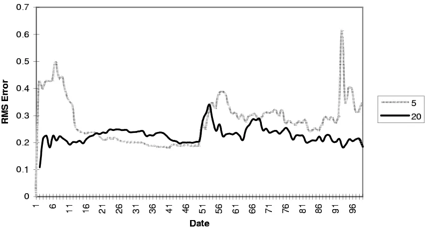
This is not the place to give the full results of this model but to give a flavour of some of the results I show the utility gained by agents with a memory of 5 and 20 models respectively where the utility curve they are learning swaps suddenly from the easy to the hard (figure 6) and visca versa (figure 7). There are also corresponding graphs for the error in their best models (figure 8 and figure 9, respectively). Note how the dynamics are not symmetrical; the first utility curve it encounters conditions the agent for when this changes. The agents had
utility
Quantity bought of product 1
easy curve
considerably more success (in terms of utility gained) going from easy to hard rather than visca versa.
Figure 7: The utility of 20-model and 5 model agents going from hard to easy utility curve
Figure 9: The RMS Error of the best model of 20 model and 5 model agents going from hard to easy utility functions
To give a flavour of the sort of models these agents develop, in run 1 of the 30-memory agent batch the agent achieved the following model by date 75: [average [[divide [[add [[constant 1.117] [amountBoughtOf 'product-2']]] [average [[amountBoughtOf 'product-2'] [constant 4.773]]]]] [min [[amountBoughtOf 'product-2'] [cutBetween [[average [[amountBoughtOf 'product-2'] [constant 4.773]]] [constant 1.044] [add [[constant 1.1 17] [amountBoughtOf 'product-2']]]]]]]]].
The purpose of this simulation is not to be an ef ficient maximiser of utility, but to model economic agents in a more credible way . It will only be vindicated (or otherwise) when compared to real economic data. However , the model does show traits found in the real world. For example, one phenomenon that is observed is that agents sometimes get “locked” into inferior models for a considerable length of time - the model implies an inferior course of action, but this course of action is such that the agent never receives disconformation of its model. Thus this remains its best model in terms of the limited data it has, so it repeats that action. If, for example, some consumers find a satisfactory brand at an early stage in the development of their tastes and then they never try any others - their (limited) experience will never disconfirm their model of what would give them most satisfaction, even when they would like other brands better.
10 Conclusion
We have described in this paper an alternative learning hypothesis according to which agents can respecify models which they find not to be correct in the sense of the rational expectations hypothesis. Because we are concerned with environments in which agents cannot conduct exhaustive searches of the information set, we have not used stochastic or statistical methods where these require valuations of the exhaustive set of mutually exclusive events. Our agents in effect know that there are events that they cannot imagine but which could occur.
This paper is intended as a first statement that our approach to modelling learning and expectations formation is formally sound, practically relevant and, within the field of simulation modelling, describes behaviour which can achieve performance no worse than standard optimization algorithms or sound game theoretic strategies. There are a number of directions in which to pursue the implied research programme.
Because of their simplicity and the small number of observed data points, we have not assumed that agents estimate the parameters of their models statistically. A natural extension of this research is to apply it to more elaborate models which would allow for this assumption.
The strength of the approach described here is that it provides a formal description of learning as modelling which, in simple examples, performs better than textbook strategies. Learning as modelling offers a trade-off between being computationally inexpensive or parsimonious in its data requirements. The less data the agent uses, the more inventive must be his modelling. We would expect increased inventiveness to be associated with more elaborate and computationally expensive metarulebases. As any economist will recognize immediately, the rational agent will always reduce both computational resources and data requirements if these can be accomplished simultaneously without loss of relevant forecasting accuracy . Consequently, ef ficient decision-making will involve this trade-of f. Simulations under a variety of alternative assumptions will inform both theoretical development and the analysis of practical alternatives in the or ganization of decision-making in conditions of complexity and uncertainty where the trade-off between computation and data acquisition is binding.
REFERENCES
[1] Arifovic, J. 1994. Learning by genetic algorithms in economic environments. Doctoral dissertation, University of Chicago, IL.
[2] Binmore, K. and L. Samuelson, 1990. Evolutionary stability in repeated games played
by finite automata. Working paper, University of Michigan, Ann Arbor, MI and
University of Wisconsin, Madison, WI.
[3] Bray, M.M. and N.E. Savin, 1986. Rational expectations equilibria, learning, and model specification. Econometrica 54, 1129-1160.
[4] Dixon, H.D., S. Moss and S. Wallis, 1995. Axelrod meets Cournot: Oligopoly and the
evolutionary metaphor Part 1. Centre for Policy Modelling Report no. 006, Centre for
Policy Modelling, Aytoun Bld., Aytoun St., Manchester, UK.
[5] Edmonds, B. in press. What is Complexity? The philosophy of complexity per se with applications to some example in evolution. In Heylighen F. & Aerts D. (eds.), The
[6] Edmonds, B., Moss, S.J. and Wallis, S. 1996. Logic, Reasoning and a Programming Language for Simulating Economic and Business Processes with Artificial Intelligent Agents. In Ein-Dor, P. (ed.) Artificial Intelligence in Economics and Management. Boston, MA: Kluwer, 221-230.
[7] Fox, J., 1994. On the necessity of probability: Reasons to believe and grounds for doubt. In Wright G. and Ayton P. (eds.). Subjective Probability. London: John Wiley.
[8] Fox, H., Krause P.J. and Elvang Goranssan M., 1993. Argumentation as a general framework for uncertain reasoning. Uncertainty in Artificial Intelligence, 8. San Mateo: Morgan Kaufmann.
[9] Halpern, J.Y. and Fagin R. 1992. Two views of belief - belief as generalized probability and belief as evidence. Artificial Intelligence, 54(3):275-317.
[10] Koza, J. 1992. Genetic Programming. Cambridge, MA: MIT Press.
[11] Lenat, D.B. 1991. On the Thresholds of Knowledge. Artificial Intelligence, 47:185-250. [12] Marimon, R., E. McGrattan and Sargent T.J. 1989. Money as a medium of exchange in
an economy with artificially intelligent agents. Journal of Economic Dynamics and
Control, 14:329-373.
[13] Masuch, M. and Huang Z. 1994. A logical deconstruction of organizational action:
formalizing Thompson’s ‘Organizations in Action’ in a multi-agent action logic.
CCSOM Working Paper 94-120,
[14] Moss, S., 1993. The economics of positive methodology. In Blackwell R., Chatta J. and Nell E., (eds.). Economics as Worldly Philosophy. Basingstoke: Macmillan.
[15] Moss, S., 1995. Control metaphors in the modelling of decision-making behaviour.
Computational Economics, 8:283-301.
[16] Moss, S. and Edmonds B. 1994. Economic methodology and computability:
implications for the evaluation of econometric forecasts. CPM Report no. 001, Centre for Policy Modelling, Aytoun Bld., Aytoun St., Manchester, UK.
[17] Moss, S. and Kuznetsova, O. 1995. Modelling the Process of Market Emergence. MODEST ‘95 (Modelling Economic and Social Transition), Warsaw.
[18] Pearl, J. 1978. On the Connection Between the Complexity and Credibility of Inferred Models. International Journal of General Systems, 4:255-264.
[19] Popper, K., 1965. Conjectures and Refutations: the growth of scientific Knowledge. New York: Harper Torchbooks.
[20] Quine, W.V. O. 1960. Simple Theories of a Complex World. In The Ways of Paradox. New York: Random House, 242-246.
[21] Wallis, S., Edmonds, B. and Moss, S.J. 1995. The Implementation and Logic of a Strictly Declarative Modelling Language, Expert Systems ‘95, Cambridge. Published as Macintosh, A. and Cooper, C. (eds.) 1995. Applications and Innovations in Expert