The Decision-Making Support For Production Planning & Supplier Selection Under Probabilistic Environment Using Bi-Objective Programming: A Single Period Case

(1)

209

The Decision-Making Support For Production

Planning & Supplier Selection Under Probabilistic

Environment Using Bi-Objective Programming: A

Single Period Case

Solikhin, Sutrisno, Purnawan Adi Wicaksono

Abstract: This article discusses the formulation of a decision-making support tool for production planning and supplier selection problem with some uncertain parameters. This involved the use of probabilistic programming with the uncertain parameter approached as a random variable. Moreover, two objective functions were optimized in the model and these include the number of products to be produce required to be maximized and the total operational cost to be minimized. The optimal decision was calculated using the probabilistic bi-objective programming in LINGO 18.0 software after which a numerical experiment was conducted to illustrate the process involved in determining the decision. The results showed the optimal supplier to be selected corresponds to the optimal number of each raw material type while the quantity of products to be produced was also determined. This, therefore, means it is possible for manufacturing industries’ actors to use this decision-making support tool.

Index Terms: bi-objective programming, decision-making support, probabilistic environment, probabilistic programming, production planning, supplier selection, supply chain management.

——————————  ——————————

1. INTRODUCTION

Manufacturing industries have several activities which are needed to be conducted optimally to obtain more profit and two of these are production planning and supplier selection. Production planning involves determining the number of each product type to be produced while supplier selection focuses on selecting the appropriate suppliers to provide the raw materials needed by the manufacturer and the quantity to be ordered. These decisions are required to reduce the total cost to be incurred but several constraints have been observed in the process with the simplest being the fulfilment of products demanded through raw materials while some other challenges are inherent in more complex problems. Several approaches have been developed to be used as decision-making support for this problem but most of them employed the mathematical optimization model such as the mixed-integer non-linear programming used to solve the supplier selection problem in [1]. A little bit more complex approach has been discussed to solve the same problem using carrier selection via mathematical programming [2], [3]. Meanwhile, the advanced problem including inventory management and was also solved using the same method [4]. All these studies involved only one objective function which was the cost and several advanced models have been developed to optimize two or more objective functions via multi-objective programming as shown in [5]. Examples of these are seen in problems such as production planning in paper mill [6], supplier selection in welding company [7], supplier selection in shipbuilding yards [8], supplier selection in electronic manufacturer [9], and

several others. These mathematical models were developed for fully known parameters which certain values. Meanwhile, there are situations in production planning and supplier selection where several parameters are unknown or uncertain and this, therefore, means they need to be solved in an uncertain environment with the mathematical model containing some uncertain parameters as discussed in this article. Optimization theory has several classes of mathematical programming from the simplest form such as linear to the most complex ones such as non-linear. Moreover, there are two types of the objective function in a model and they include single and multi-objective programming. Several cases have, however, been reported have been solved using multi-objective programming such as power source [10]–[15],

mechanical system [16], water management [17],

pharmaceutical production [18], physical reactor plant [19], train ventilation [20], schedule management [21], and others. This type, theoretically, solves problems by determining the Pareto solution through the use of some approaches like weighting [22]. The working principle of Pareto optimality is shown in case study articles such as those conducted on battery cell [23], re-insurance [24]–[26], and radar [27]. A decision-making support tool was formulated in this article via probabilistic multi-objective programming for production planning and supplier selection problem which contains several uncertain parameters approached as probabilistic parameters with some probability distribution function. Moreover, numerical experiments were conducted to evaluate the model and observe the process involved in making the decision.

2 DECISION-MAKING

TOOL:

MATHEMATICAL

MODEL

2.1 Problem Definition

A decision-maker in a production unit wants to produce a quantity of product types P from R quantity of raw materials to be purchased from S number of suppliers. The variables to be decided include the quantity of each raw material to be ————————————————

 Solikhin is currently as part of Dept. of Mathematics, Diponegoro University, Indonesia as lecturer and researcher. E-mail: [email protected]

 Sutrisno is currently as part of Dept. of Mathematics, Diponegoro University, Indonesia as lecturer and researcher. E-mail: [email protected]

 Purnawan Adi Wicaksono is currently as part of Dept. of Industrial Engineering, Diponegoro University, Indonesia as lecturer and researcher. E-mail: [email protected]

(2)

210 ordered from each supplier and the quantity of each product to

be produced in order to satisfy demand. Some of the uncertain conditions to be resolved are as follow:

TABLE1

MATHEMATICAL NOTATIONS:INDEX

Symbol Interpretation

r Index notation for raw material type 1, 2, ..., R s Index notation for supplier 1, 2,..., S

p Index notation for product type 1, 2, …, P TABLE2

DECISION VARIABLE Symbol Interpretation

p

Y Quantity of product p to be produced p

YR Quantity of product p decided to be procured after the

random variables are revealed sr

X Quantity of raw material r to be purchased to supplier

s s

Z Assignment variable for supplier s (equals 1 if

purchasing raw material to supplier s or 0 if no raw material purchased to supplier s)

s

TR Number of trucks to be used to deliver the raw

materials from supplier s TABLE3

PROBABILISTIC PARAMETERS

sr

UP Random variable declaring the price for one-unit raw

material r to be purchased from supplier s sr

DR Random variable declaring the percentage of

defected raw materials r due to damage from supplier s

sr

SR Random variable declaring the percentage of raw

materials r shortage from supplier s p

DE Random variable declaring the demand value for

product p p

DRY Random variable declaring the percentage of

underqualified product p produced TABLE4

DETERMINISTIC PARAMETERS

p

DRY Random variable declaring the percentage of

underqualified product p produced p

YRP Price per unit for recourse product p to satisfy the

demand if the produced products are less than the demand

s

OC Ordering cost to supplier s s

TC Transportation cost per one truck to deliver raw

materials from supplier s sr

PD Penalty cost for one unit of defected raw material

r from supplier s sr

PS Penalty cost for one unit of raw material r

shortage from supplier s rp

RP Number of raw material r required to produce one

unit of product p pm

MH Hour resource to machine m required to produce

one unit of product p m

MM Maximum capacity of hour resource for machine

m operated for production p

PC Cost to produce one unit of product p p

DCY Penalty cost for one unit of defected product p MR Maximum capacity of one truck to transport raw

material sr

MS Maximum capacity of the supplier s to supply raw

material r

1) It is possible some raw materials are defected due to damage while transporting or their quality may not be acceptable when they are delivered. This number was assumed to be uncertain.

2) It is possible some raw materials ordered are delivered late due to a lot of factors such as delivery service disturbance, shortage on the supplier, etc. The number was also considered uncertain.

3) It is possible some products from the production unit or manufacturer are defected or not up to quality. The quantity was also assumed to be uncertain.

4) The quantity of qualified product is expected to satisfy the demand value which was assumed to be uncertain 5) The capacity of the trucks was assumed to be equal The other applicable conditions are explained in the mathematical model and the decision variables were calculated to reduce the operational cost and maximize the quantity of products.

2.2 Mathematical Model

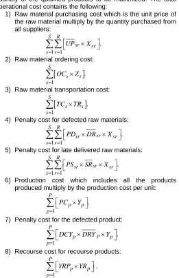
The symbols used in the mathematical model are shown in Table 1 to Table 4 and the two objective functions formulated include the total operational cost to be minimized and the quantity of the qualified products to be maximized. The total operational cost contains the following:

1) Raw material purchasing cost which is the unit price of the raw material multiply by the quantity purchased from all suppliers: 1 1 . S R sr sr s r UP X       



2) Raw material ordering cost:





1 . S s s s OC Z  



3) Raw material transportation cost:





1 . S s s s TC TR  



4) Penalty cost for defected raw materials:

1 1 . S R sr sr sr s r

PD DR X

 

   

 



5) Penalty cost for late delivered raw materials:

1 1 . S R sr sr sr s r

PS SR X

 

   

 



6) Production cost which includes all the products produced multiply by the production cost per unit:

1 . P p p p PC Y      



7) Penalty cost for the defected product:

1 . P p p p p

DCY DRY Y



   

 



8) Recourse cost for recourse products:

1 P p p p YRP YR      



.

(3)

211 1 P p p Y 



.

The following conditions are required to be satisfied to optimize the previously stated objective functions:

1) The available raw materials are expected to satisfy the requirement to produce the products and this was calculated by ensuring the result of the raw materials purchased from all suppliers minus the defected ones minus the shortage is greater than the quantity needed to produce and this was formulated as:

1 1 1

1

, 1, 2,..., .

S S S

sr sr

sr sr sr

s s s

P

rp p

p

X DR X SR X

RP Y r R

         _  _ _  _    _  _  



2) The available products are expected to satisfy demand such that the manufactured product quantity plus the recourse product quantity is greater than the demanded quantity and this was formulated as:

, 1, 2,..., . p

p p

Y YR DE  p P

3) The available machine working hour used for production need to be able to satisfy the maximum capacity and this was formulated as:

1

, 1, 2,..., ; P

pm p m

p

MH Y MM m M



    

 



4) The raw material loaded for delivery is expected to satisfy the truck’s capacity and this was formulated as:

1 _, _{1, 2,..., ,}

R

r sr

s X

TR s S

MR  _       _{ }        



where  _{ }. denotes a floor function.

5) The quantity of raw material purchased from a supplier is expected to be less than the supplier’s maximum capacity to supply the corresponding raw material and this was formulated as:

, 1, 2,..., , 1, 2,..., ;

sr sr

X MS  s S  r R

6) The constraint to determine the selection of a supplier was formulated as:

1

1, if 0,

1, 2,..., ;

0, otherwise, R

sr

s r

X

Z _ s s

   _    



7) The constraints to assign the decision variables are integer and nonnegative and formulated as:

 

, , , 0 and integer, 0,1 .

sr p p s s

X Y YR TR  Z 

 

0,1 s

W  .

Let E

 



be the expectation value of the random variable .



Then, it is possible to formulate the whole optimization as the following probabilistic bi-objective optimization problem:

1 1 max P p p Z Y 





(1)









2 1 1 1 1 1 1 1 1 1 1 min S R sr sr s r S R sr sr sr s r S R sr sr sr s r S S

s s s s

s s

P P

p

p p p p

p p

Z E X UP

PD DR X

PS SR X

OC Z TC TR

PC Y DCY DRY Y

               _  _     _   _     _              _  _ _   _





1 P p p p YRP YR   





_  _ (2)

subject to:

1 1 1

1

, 1, 2,..., ;

S S S

sr sr

sr sr sr

s s s

P

rp p

p

X E DR X SR X

RP Y r R

            _  _ _  _        _  _ 



, 1, 2,..., ; p

p p

Y YR E DE_ _  p P

1

, 1, 2,..., ; P

pm p m

p

MH Y MM m M



    

 



1 _, _{1, 2,..., ;}

R sr r

s X

TR s S

MR       _{ }          



, 1, 2,..., , 1, 2,..., ;

sr sr

X MS  s S  r R

1

1, if 0,

1, 2,..., ;

0, otherwise, R

sr

s _r

X

Z _ s s

       



 

, , , 0 and integer, 0,1 ; {0,1}.

sr p p s s s

X Y YR TR  Z  W 

This problem was solved using a deterministic equivalent approach by generating its optimization model and the feasible solution set, if not empty, was closed and bounded. Therefore, the optimization was well defined and the existence of the optimal solution was guaranteed. Furthermore, maxZ₁ was

replaced with ₁

1 minZ  



P_p_Y_p .

Pareto was applied to solve this bi-objective optimization

and this involved using a vector of decision variables xo to

ensure there was no other vector x to make

Z x

_i

( )



Z x

_i

(

o

)

,

1, 2 i

(4)

212

1 1 2 2

minZw(Z )w Z , (3)

subject to: w₁w₂1, 0w w₁, ₂1.

3 NUMERICAL

EXPERIMENT

A numerical experiment was considered to illustrate the problem in Section 2 with the three types of raw material denoted by R1, R2 and R3, four suppliers denoted by S1, S2, S3 and S4, and three product types denoted by P1, P2 and P3. Let N( , )a b denote a normal probability distribution

function with mean a and variance b. The value for crisp parameters is provided in the appendix with the probability distribution of the random variables shown in Table 5 while the values of the remaining parameters are presented from Table 6 to 14.

TABLE5

PROBABILITY DISTRIBUTION FUNCTION FOR PROBABILISTIC PARAMETERS

Probabilistic Parameter Probability distribution sr

UP N(5, 2)

sr

DR N(0.05, 0.02)

sr

SR N(0.05, 0.02)

p

DE N(100,10)

p

DRY N(0.05,0.01)

TABLE6

PRODUCTION COST AND DEFECT PRODUCT COST Supplier Production cost Defect product cost

P1 2 1

P2 2 1

P3 3 1

TABLE7

ORDER COST AND TRANSPORT COST

Supplier Order Cost Transport Cost

S1 50 80

S2 20 100

S3 40 105

S4 20 95

TABLE8

DEFECT PRODUCT PENALTY COST

Supplier Raw Material

R1 R2 R3

S1 1 2 4

S2 2 2 5

S3 1 3 5

S4 1 2 5

TABLE9

RAW MATERIAL SHORTAGE PENALTY COST

R1 R2 R3

S1 0.5 1 2

S2 0.2 1.5 2.5

S3 0.2 1 2

S4 0.5 1.5 2

TABLE10

RAW MATERIAL REQUIRED TO PRODUCE THE PRODUCT

Raw Material Product

P1 P2 P3

R1 1 2 1

R2 1 1 1

R3 2 1 1

TABLE11 SHORTAGE COST

Product Shortage cost Raw Material Shortage cost

P1 4 R1 2

P2 3 R2 3

P3 4 R3 2

TABLE12

REQUIRED MACHINE WORKING HOUR TO PRODUCE PRODUCT UNIT

Product Machine

M1 M2 M3

P1 0.5 0.5 1

P2 0.2 0.2 0.1

P3 0.4 0.2 0.1

The optimal decision was calculated by solving (3) with

1 2 0.5

w w  which means the weight for the objective function Z₁ and Z₂ is uniform and there is no priority between them. This was calculated using LINGO 18.0 software in a commonly used personal computer with a 3.2 GHz processor and 4 GB memory. The number of core variables was 28 and its deterministic equivalent was 112 while the number of core constraints was 32 and its deterministic equivalent was 185. The number of scenarios was 4 with the number of random variables being 42. The computational time was very fast and was able to solve the problem at about only 1 second.

TABLE13

MACHINE WORKING HOUR MAX.CAPACITY

M1 M2 M3

4500 4500 5000

TABLE14

SUPPLIER MAXIMUM CAPACITY TO SUPPLY RAW MATERIAL

R1 R2 R3

S1 850 850 500

S2 800 850 400

S3 800 500 500

(5)

213 From Fig. 1a, it shows that the optimal decision for raw material procurement was to order 53 units of R1, 313 of R2, and 399 of R3 from supplier S2, and 355 of R1, 8 of R2, and 33 of R3 from S3 while S1 and S4 are not to be selected. Moreover, Fig. 1b shows the optimal decision for the production planning with 109 units of P1, 77 of P2, and 100 of P3 expected to be produced. Therefore, the optimal objective value of Z1 representing the total production number was 280. Fig. 2 shows the optimal objective value of Z2 indicating the expectation of operational cost was 77630 for scenario-1, 90040 for scenario-2, 76600 for scenario-3, and 70650 for scenario-4. The recourse product for scenario-1 was 20 units of P2 and this means in a situation the demand value is 96 units 77 units of P2 produced would not satisfy the demand and the 19 units shortage replaced by the 20 units of the recourse. The other scenarios are interpreted as the same. Meanwhile, in case the products are unable to satisfy the demand, the decision-maker does not have to purchase recourse products and this has the possibility of causing a loss of revenue from selling the product.

4 CONCLUDING

REMARKS

AND

FURTHER

WORKS

A decision-making support tool via probabilistic bi-objective mathematical model was developed to measure the optimal decision for supplier selection and production planning problem. This involved using the probabilistic programming implemented n LINGO 18.0 optimization software. Moreover, a numerical experiment was conducted with three types of raw material purchased from four suppliers, and three types of products. An optimal decision was obtained and this shows the decision-making tool is reliable to be applied by actors in the manufacturing industries. Further works are expected to deal with more complicated problems developed from the findings of this study, especially the multi-period case such as the

Fig. 2. Objective value, recourse product amount, and demand amount for scenario 1, 2, 3, and 4

(a)

(b)

Fig. 1. (a) The optimal decision for raw material procurement for each R1, R2, and R3 (b) The optimal decision for the amount of product P1, P2, and

(6)

214 inventory management with the raw materials and products

stored in a warehouse for future use.

ACKNOWLEDGMENT

The authors appreciate the Universitas Diponegoro for providing the research funding via RPI 2020 research grant contract no. 233-27/UN7.6.1/PP/2020.

REFERENCES

[1] N. R. Ware, S. P. Singh, and D. K. Banwet, ―Expert Systems with Applications A mixed-integer non-linear program to model dynamic supplier selection problem,‖ Expert Syst. Appl., vol. 41, no. 2, pp. 671–678, 2014, doi: 10.1016/j.eswa.2013.07.092.

[2] D. Choudhary and R. Shankar, ―Joint decision of procurement lot-size, supplier selection, and carrier selection,‖ J. Purch. Supply Manag., vol. 19, no. 1, pp. 16–26, 2013, doi: 10.1016/j.pursup.2012.08.002.

[3] D. Choudhary and R. Shankar, ―A goal programming model for joint decision making of inventory lot-size, supplier selection and carrier selection,‖ Comput. Ind. Eng., vol. 71, no. 1, pp. 1–9, 2014, doi: 10.1016/j.cie.2014.02.003.

[4] D. U. H. E. Hakim, Sutrisno, and Widowati, ―Quadratic programming model for optimal decision making of supplier selection problem integrated with inventory control problem,‖ J. Phys. Conf. Ser., vol. 1217, no.

12060, pp. 1–10, 2019, doi:

10.1088/1742-6596/1217/1/012060.

[5] A. Trivedi, A. Chauhan, S. P. Singh, and H. Kaur, ―A multi-objective integer linear program to integrate supplier selection and order allocation with market demand in a supply chain,‖ Int. J. Procure. Manag., vol. 10, no. 3, pp. 335–359, 2017, doi: 10.1504/IJPM.2017.083466.

[6] J. Mattila, V. Hotti, and M. Juhola, ―Product mix and its optimisation in a paper mill according to the profitability computation of process measurements,‖ Int. J. Comput. Aided Eng. Technol., vol. 3, no. 2, pp. 155–174, 2011, doi: 10.1504/IJCAET.2011.038824.

[7] S. Sarkar, D. K. Pratihar, and B. Sarkar, ―An integrated fuzzy multiple criteria supplier selection approach and its application in a welding company,‖ J. Manuf. Syst., vol. 46, pp. 163–178, 2018, doi: 10.1016/j.jmsy.2017.12.004. [8] J. Li et al., ―Semantic multi-agent system to assist

business integration: An application on supplier selection for shipbuilding yards,‖ Comput. Ind., vol. 96, pp. 10–26, 2018, doi: https://doi.org/10.1016/j.compind.2018.01.001. [9] C. Pornsing, P. Jomtong, J. Kanchana-anotai, and T.

Tonglim, ―Solving Supplier Selection Problem Using Fuzzy-AHP for An Electronic Manufacturer,‖ in 2019 IEEE 6th International Conference on Industrial Engineering and Applications (ICIEA), 2019, pp. 824–827, doi: 10.1109/IEA.2019.8715115.

[10] H. M. G. C. Branco, M. Oleskovicz, D. V. Coury, and A. C. B. Delbem, ―Multiobjective optimization for power quality monitoring allocation considering voltage sags in distribution systems,‖ Int. J. Electr. Power Energy Syst., vol. 97, no. November 2017, pp. 1–10, 2018, doi: 10.1016/j.ijepes.2017.10.011.

[11] E. B. Schlünz, P. M. Bokov, and J. H. van Vuuren, ―Multiobjective in-core nuclear fuel management optimisation by means of a hyperheuristic,‖ Swarm Evol. Comput., no. November 2017, pp. 1–19, 2018, doi:

10.1016/j.swevo.2018.02.019.

[12] H. Rashidi and J. Khorshidi, ―Exergy analysis and multiobjective optimization of a biomass gasification based multigeneration system,‖ Int. J. Hydrogen Energy, vol. 43, no. 5, pp. 2631–2644, 2018, doi: 10.1016/j.ijhydene.2017.12.073.

[13] K. Yu et al., ―Multiobjective optimization of ethylene

cracking furnace system using self-adaptive

multiobjective teaching-learning-based optimization,‖ Energy, vol. 148, pp. 469–481, Apr. 2018, doi: 10.1016/J.ENERGY.2018.01.159.

[14] F. Ruiming, ―Multi-objective optimized operation of integrated energy system with hydrogen storage,‖ Int. J.

Hydrogen Energy, 2019, doi:

https://doi.org/10.1016/j.ijhydene.2019.02.168.

[15] A. Zendehboudi, A. Mota-Babiloni, P. Makhnatch, R. Saidur, and S. M. Sait, ―Modeling and multi-objective optimization of an R450A vapor compression refrigeration system,‖ Int. J. Refrig., vol. 100, pp. 141–155, 2019, doi: https://doi.org/10.1016/j.ijrefrig.2019.01.008.

[16] J. F. A. Madeira, A. L. Araújo, C. M. Mota Soares, and C. A. Mota Soares, ―Multiobjective optimization for vibration reduction in composite plate structures using constrained layer damping,‖ Comput. Struct., 2017, doi: 10.1016/j.compstruc.2017.07.012.

[17] K. Zhang, H. Yan, H. Zeng, K. Xin, and T. Tao, ―A practical multi-objective optimization sectorization method for water distribution network,‖ Sci. Total Environ., vol.

656, pp. 1401–1412, 2019, doi:

https://doi.org/10.1016/j.scitotenv.2018.11.273.

[18] S. Liu and L. G. Papageorgiou, ―Multi-objective optimisation for biopharmaceutical manufacturing under uncertainty,‖ Comput. Chem. Eng., vol. 119, pp. 383–393,

2018, doi:

https://doi.org/10.1016/j.compchemeng.2018.09.015. [19] P. Chaudhari and S. Garg, ―Multi-objective optimization of

maleic anhydride circulating fluidized bed (CFB) reactors,‖ Chem. Eng. Res. Des., vol. 141, pp. 115–132, 2019, doi: https://doi.org/10.1016/j.cherd.2018.10.020. [20] N. Li, L. Yang, X. Li, X. Li, J. Tu, and S. C. P. Cheung,

―Multi-objective optimization for designing of high-speed train cabin ventilation system using particle swarm optimization and multi-fidelity Kriging,‖ Build. Environ., 2019, doi: https://doi.org/10.1016/j.buildenv.2019.03.021. [21] H. Ahmadi-Nezamabad, M. Zand, A. Alizadeh, M.

Vosoogh, and S. Nojavan, ―Multi-objective optimization based robust scheduling of electric vehicles aggregator,‖ Sustain. Cities Soc., vol. 47, p. 101494, 2019, doi: https://doi.org/10.1016/j.scs.2019.101494.

[22] J. Branke, K. Deb, K. Miettinen, and R. Slowinski, Multiobjective Optimization: Interactive and Evolutionary Approaches. Berlin: Springer-Verlag Berlin Heidelberg, 2008.

[23] Y. Hong and C. W. Lee, ―Pareto fronts for multiobjective optimal design of the lithium-ion battery cell,‖ J. Energy Storage, vol. 17, no. April, pp. 507–514, 2018, doi: 10.1016/j.est.2018.04.003.

[24] X. Zeng and S. Luo, ―Stochastic Pareto-optimal reinsurance policies,‖ Insur. Math. Econ., vol. 53, no. 3,

pp. 671–677, 2013, doi:

10.1016/j.insmatheco.2013.09.006.

(7)

215

Econ., vol. 77, pp. 24–37, 2017, doi:

10.1016/j.insmatheco.2017.08.004.

[26] A. V. Asimit, V. Bignozzi, K. C. Cheung, J. Hu, and E. S. Kim, ―Robust and Pareto optimality of insurance contracts,‖ Eur. J. Oper. Res., vol. 262, no. 2, pp. 720– 732, 2017, doi: 10.1016/j.ejor.2017.04.029.