Selection and Construction of Six Sigma TNT
Variables Sampling Scheme
(n
σ
; k
T
, k
N
) indexed by Six Sigma Quality
Levels
Dr. B. Esha Raffie1 and Dr. D. Senthilkumar2
1
Assistant Professor, PSG College of Arts & Science, Coimbatore – 641 014.
2
Head & Associate Professor, PSG College of Arts & Science, Coimbatore – 641 014.
Abstract
This article gives selection of Six Sigma Tightened- Normal – Tightened Variables Sampling Scheme (SSTNTVSS (nσ; kT, kN)) indexed by Six Sigma
AQL and Six Sigma AOQL. The procedure of tables constructed for easy selection of system given indexed by six sigma quality levels by known and unknown σ at Six Sigma levels.
Keywords - Tightened- Normal – Tightened Scheme, Variables Sampling, Six Sigma AOQ, Six Sigma AQL and Six Sigma AOQL.
I. INTRODUCTION
A lot- by – lot rectifying inspection scheme for a series of lots calls for 100% inspection of rejected lots under application of sampling plan. If one prefers to use a single sampling plan for variables under a rectification inspection scheme, the quality indicator for the selection of the sampling plan will be the average outgoing quality limit (AOQL), which is the worst average quality the consumer will receive in the long run, no matter what the incoming quality is. Rejected lots are often a nuisance to the producer as they result in extra work and cost. If too many lots are rejected, this will damage the reputation of the producer or supplier. From the producer point of view, he would prefer fixing an acceptable quality level (AQL) and designing sampling plan so that if the incoming product quality is maintained at AQL, most of his lot (say 99.9%) will be accepted during the sampling inspection stage itself. Thus, designing sampling inspection plan indexed by SSAQL and SSAOQL satisfies both the producer and consumer whenever rectifying inspection is necessary. Soundararajan (1981) has developed procedures and tables for the selection of single sampling plans for attributes for given AQL and AOQL. Govindaraju (1990) has developed procedures and tables for the selection of single sampling plans for variables indexed by AQL and AOQL. Later Soundarajan and Palanivel (2000) have developed procedures and tables for the selection of quick switching single sampling variables systems indexed by AQL and AOQL. Based on above article Senthilkumar and
Esha Raffie (2017) have constructed SSQSVSS (nσ;
kTσ, kNσ) indexed by Six Sigma AQL and Six Sigma
AOQL. Senthilkumar and Esha Raffie (2018) have constructed six sigma modified quick switching variables sampling system [SSMQSVSS-r (nTσ, nNσ;
kσ), r=2 and 3] indexed by six sigma quality levels of
SSAQL and SSAOQL. Muthuraj and Senthilkumar
(2006) have developed the procedures and
constructed tables for the selection of tightened – normal – tightened variables sampling scheme indexed by AQL and AOQL. This concept can be extended to variables quality characteristics of the study, the resulting plan would be designated as SSTNTVSS and would be applied under the following conditions:
i) Production is steady so that results on current, preceding and succeeding lots are broadly indicative of a continuing process. ii) Lots are submitted substantially in the order of production.
iii) Inspection is by variables, with quality of an individual item defined in terms of fraction defective.
A. Basic assumptions
a) The quality characteristics is represented by a random variable X measurable on a continuous scale.
b) Distribution of X is normal with mean µ and standard deviation σ.
c) An upper limit U, has been specified and a product is qualified as defective when X>U.[when the lower limit L is specified, the product is a defective one if X<L]. d) The Purpose of inspection is to control the
fraction defective, p in the lot inspected. When the conditions listed above are satisfied the fraction defective in a lot will be defined by
p = 1 -F (v )= F (-v ) with v =μ ) / σ( and U
2 / 2
1 F ( y )
2
z
e d z
1
y
(1)
where z ~ N (0, 1). Here the decision criterion for the σ- method variables plan is to accept the lot if
X + k σ ≤ U , where U is the upper specification
limit or if X + k σ ≥ L , where L is the lower specification limit.
B. SSTNTVSS with known σ variable plan as the reference plan
The operating procedure of SSTNTVSS(nσ; kTσ, kNσ)
are described below.
Step 1: Inspect under tightened inspection using the single sampling plan with sample size nTσ
and the acceptance constant kT.Accept the
individual lot, if
T T
X + k σ U o r X - k σ Lwhere X is the
sample mean. If t lots in a row are accepted, switch to normal inspection (Step 2).
Step 2: Inspect under normal inspection using the single sampling plan with sample size nNσ
and the acceptance constant kN.Reject the
individual lot, if
N N
X + k σ U o r X - k σL where X is
the sample mean. When an additional lot is rejected in the next s lots after a rejection, switch to tightened inspection.
Thus, a SSTNTVS scheme where tightening is based on the acceptance constants is specified by the parameters nσ, kTσ, kNσ, s and t, where nσ is the
sample size and kNσ and kTσ are the acceptance
constants of the variables sampling plan under normal and tightened inspection respectively, t is the criterion for switching to normal inspection, and s is the criterion for switching to tightened inspection. The Six Sigma TNT variables sampling scheme is simply designated as SSTNTVSS (nσ; kTσ, kNσ).
When s =4 and t = 5, the OC function of the TNTVSS becomes the scheme OC function of MIL – STD – 105D that involves tightened and normal inspections was derived by Dodge (1965), Hald and Thyregod (1965) and Stephen and Larson (1967).
II. OPERATING CHARACTERISTIC FUNCTION
According to Calvin (1977), the OC function of the TNT scheme is given by
Pa p
=PT 1 − PN
S 1 − P
Tt 1 − PN + PNPTt 1 − PT 2 − PNS
1 − PNS 1 − PTt 1 − PN + PTt 1 − PT 2 − PNS
(2)
where PT and PN are the proportion of lots expected to
be accepted using tightened (nσ, kT) and normal (nσ,
kN) variables single sampling plans respectively.
Under the assumption of normal distribution, the expression for PT and PN are given by
PT = Pr [(U –X )/σ ≥ kT] (3)
And
PN = P [(U –X )/σ ≥ kN] (4)
respectively. Equations (3) and (4) are substituted in (2) to find Pa(p) values for given p, s, t, n, kT, and kN.
As the individual values of X follows normal distribution with mean µ and variance σ2
, the expressions given in (8.3) and (8.4) can be restated as
T
2 ( - z / 2 ) T
1
P e d z
2
w
andN
2 ( - z / 2 ) N
1
P e d z
2 w
respectively, withT T T
w = n ( U -k σ -μ ) / σ = ( v -k ) n ,
N N N
w = n ( U -k σ -μ )/σ = (v -k ) n and
ν = (U - μ ) / σ
To determine the values of nσ, kTσ, and kNσ the
given values of p1, p2, α and β should satisfy the
following two equations. That is,
𝑃𝑎 𝑝
=𝑃𝑇 1 − 𝑃𝑁
𝑆 1 − 𝑃
𝑇𝑡 1 − 𝑃𝑁 + 𝑃𝑁𝑃𝑇𝑡 1 − 𝑃𝑇 2 − 𝑃𝑁𝑆
1 − 𝑃𝑁𝑆 1 − 𝑃
𝑇𝑡 1 − 𝑃𝑁 + 𝑃𝑇𝑡 1 − 𝑃𝑇 2 − 𝑃𝑁𝑆
(5)
III. SSAOQL PROCEDURES
If the quality of the accepted lot is p and all defective units found in the rejected lots are replaced by non-defective units in a rectifying inspection plan, the Six Sigma average outgoing quality (SSAOQ) can be approximated as
SSAOQ = pPa(p) (6)
Where Pa(p)is defined in the equation (2). If
pm is the proportion nonconforming items at which
SSAOQ is maximum, one has
SSAOQL = pmPa(pm) (7)
If SSAQL (p1) is prescribed, then the
corresponding value of vSSAQL or v1 will be fixed and
if Pa(p) is fixed at 99.99966%, that is (1-α). Where, α
= 0.0000034x10⁻⁶. Hence we have
Pa(p1) = (1-α) which is obtained from equation (5),
and v1 satisfies
wN = (v1 – kNσ) nσ (8)
and wT = (v1 – kTσ) nσ (9) so that for given values of nσ, wN, wT and SSAQL,
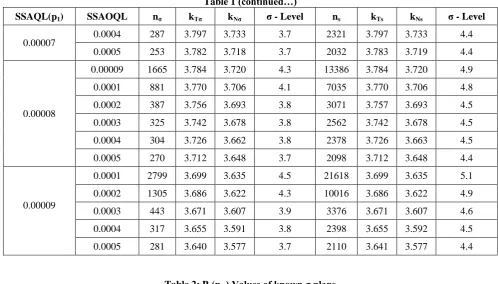
A. Selection of known σ SSTNTVSS(nσ; kTσ, kNσ) for
given SSAQL and SSAOQL
Table 1 is used for selection of σ- method SSTNTVSS. For example, if the SSAQL is fixed at p1=0.00009 and the SSAOQL is fixed at 0.0001,
Table 1 yields nσ = 2799, kTσ = 3.699 and kNσ = 3.635,
which is associated with 4.5 sigma level of SSTNTVSS (nσ; kTσ, kNσ).
The user of Table 1 should understand the limitations of plans indexed by SSAOQL. Sampling with rectifying of rejected lots on the one hand reduces the average percentage of nonconforming items in the lots, but on the other hand introduces non-homogeneity in the series of lots finally accepted. That is, any particular lot will have a quality of p% or 0% nonconforming depending on whether the lot is accepted or rectified. Thus the assumption underlying the SSAOQL principle is that the homogeneity in the qualities of individual lots is unimportant and only the average quality matters. For plans listed in Table 1, if the individual lot quality happens to be the product quality pm at which SSAOQL occurs, then the
associated probability of acceptance will be poor. Table 2 gives Pa(pm) values of plans given in Table 1.
For example, for SSAQL of p1=0.00004 and
SSAOQL =0.0002, Table 8.3 gives Pa(pm) = 0.67.
Then pm = SSAOQL/ Pa(pm) = 0.00037. In order to
avoid such inconvenience, the producer should maintain the process quality more or less at the SSAQL. The high rate of rejection of lots at p = pm
will also indirectly put pressure on the producer to improve the submitted quality.
B. Selection of unknown σ SSTNTVSS(nσ; kTσ, kNσ)
for given SSAQL and SSAOQL
Table 1 also gives such matched S-method plan. For example, for given SSAQL of p1=0.00007
and SSAOQL 0.0003, one obtains the parameters of the S-method plan from Table 5.2 to be ns = 2509, kTσ
= 3.813 and kNσ = 3.749, which is associated with 4.5
sigma level of SSTNTVSS(nσ; kTσ, kNσ).
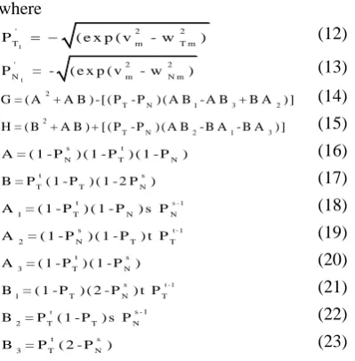
IV. CONSTRUCTION OF TABLE 1 AND 2
For constructing Table 1, a trial value of pm is
assumed and the probability of acceptance at pm is
found using (6) as
Pa(pm) = SSAOQL / pm (10)
The auxiliary variables vm, wNm and wTm
corresponding to the values of pm and Pa(pm)
respectively, are found using (1) to (4). For given values of p1, determine the values of v1, wN and wT
using the approximation (Abramwitz and Stegun (1972)) for the ordinate of the cumulative normal distribution. With the values of vm, wNm and wTm, the
following equations are derived which Muthuraj and Senthilkumar(2006) used for calculating nσ.
1
2 ' ' 2
σ m T N
n = (-A O Q L ) / (p (P GP H ) / (A + B ) (11)
where
1
' 2 2
T m T m
P ( e x p ( v - w ) (12)
1
' 2 2
N m N m
P = - ( e x p ( v - w ) (13)
2
T N 1 3 2
G = ( A + A B ) - [ ( P - P ) ( A B - A B + B A ) ] (14)
2
T N 2 1 3
H = ( B + A B ) + [ ( P - P ) ( A B - B A - B A ) ] (15)
s t
N T N
A = ( 1 - P ) ( 1 - P ) ( 1 - P ) (16)
t s
T T N
B = P ( 1 - P ) ( 1 - 2 P ) (17)
s - 1
t
1 T N N
A = ( 1 - P ) ( 1 - P ) s P (18)
t - 1
s
2 N T T
A = ( 1 - P ) ( 1 - P ) t P (19)
t s
3 T N
A = ( 1 - P ) ( 1 - P ) (20)
t - 1
s
1 T N T
B = ( 1 - P ) ( 2 - P ) t P (21)
t s - 1
2 T T N
B = P ( 1 - P ) s P (22)
t s
3 T N
B = P ( 2 - P ) (23)
Equation (11) is the formula for finding the sample size of a known σ SSTNTVSS. With the values of nσ
obtained from (11), it is then checked to see whether the assumed value of pm corresponds to the proportion
non-conforming at which the SSAOQL occurs or not. That is, it is checked to see whether or not the trial value of pm satisfies the following condition.
1
2 ' ' 2
m T N
A O Q L + [(p (P GP H ) / (A + B ) ]0 (24)
where 1
' 2 2
T σ m T m
P n e x p ( v - w ) (25)
1
' 2 2
N σ m N m
P = - n e x p ( v - w ) (26)
The value of G, H, A and B are obtained from equation (14) to (15). The Equation (24) was obtained from the following relation
d P ( p )
d ( S S A O Q ) a
= P ( p ) + pa = 0
d p d p (27)
in which
T N
2
' '
P G + P H
d ( S S A O Q ) =
d p ( A + B )
(28)
If assumed value of pm does not satisfy (27),
then another trial value of pm is obtained from (27) by
numerical methods. The methods of successive substation is often found to give good results and (27) is rewritten for this purpose as
T N
2
' '
pm= ( -A O Q L ) /[ pm( P G + P H ) /( A + B ) ] (29)
After determining the next trial value of pm,
again the values of vm, wNm, wTm and nσ are found and
the condition (24) rechecked. This iterative procedure continues until the convergence of pm is achieved.
Then the value of kNσ and kT σ are obtained from (3)
For obtaining the values of v1, wN and wT,
the approximation for the ordinate of the cumulative normal distribution available in Abramowitz and Stegun (1972) was used.
The S-method plans matching the σ-method plans were obtained using computer search routine through C++ programme. For selected combinations of SSAQL and SSAOQL, Table 1 was constructed following the above iterative procedure.
REFERENCES
[1] D.J.Sommers, Two-point double variables sampling plans, Journal of Quality Technology, 13(1981).
[2] D.Muthuraj and D. Senthilkumar, Contributions to the Study of Certain Variables and Attributes Sampling Schemes and Plans, Phd thesis, Bharathiar University.
[3] D.Senthilkumar and B.Esha Raffie, Modified Quick Switching Variables Sampling System indexed by Six sigma Quality Levels, International Journal of Scientific Research in Science, Engineering and Technology, 3 (6) 332 - 337, 2018.
[4] D.Senthilkumar and B.Esha Raffie, Quick Switching Variables Sampling System Indexed by Six Sigma AQL and Six Sigma AOQL, International Journal of Current Research in Science and Technology, 3(10) (2017), 21-28.
[5] D.Senthilkumar and B.Esha Raffie, Six Sigma Quick Switching Variables Sampling System Indexed by Six Sigma Quality Levels, International Journal of Computer Science & Engineering Technology, 3(12) (2012), 565-576.
[6] H.F.Dodge, A New Dual System of Acceptance Sampling Technical Report, No.16, The Statistics Center, Rutgers-The State University, New Brunswick, NJ, (1967).
[7] K.Govindaraju, Single sampling Plans for Variables Indexed by AQL and AOQL, Journal of Quality Technology, 22(4) (1990), 310-313.
[8] L.D.Romboski, An Investigation of Quick Switching Acceptance Sampling Systems, Doctoral Dissertation, Rutgers the State University, New Brunswick, New Jersey, (1969).
[9] M.Abramowitz and I.A.Stegun, Handbook of Mathematical functions, Dover Publications, New York, (1972).
[10]V.Soundarajan and M.Palanivel, Quick Switching Variables Single Sampling (QSVSS) System indexed by AQL and AOQL, Journal of Applied Statistics, 27(7) (2000), 771-778.
[11]V.Soundararajan, Single Sampling Attributes Plans Indexed by AQL and AOQL, Journal of Quality Technology, 13(3)(1981), 195-200.
Table 1: SSQSVSS with known and unknown σ indexed by SSAQL and SSAOQL
SSAQL(p1) SSAOQL nσ kTσ kNσ σ - Level ns kTs kNs σ - Level
0.00001
0.00002 1112 4.345 4.281 4.2 11455 4.345 4.281 4.9
0.00003 991 4.332 4.268 4.1 10153 4.332 4.268 4.8
0.00004 878 4.317 4.253 4.1 8939 4.317 4.253 4.8
0.00005 739 4.305 4.241 4.0 7486 4.305 4.241 4.8
0.00006 587 4.294 4.230 3.9 5917 4.294 4.230 4.7
0.00007 422 4.279 4.215 3.8 4227 4.279 4.215 4.6
0.00008 244 4.264 4.200 3.6 2429 4.264 4.200 4.4
0.00009 254 4.251 4.187 3.6 2515 4.251 4.188 4.4
0.0001 243 4.236 4.172 3.6 2390 4.236 4.173 4.4
0.0002 217 4.221 4.157 3.6 2121 4.221 4.158 4.4
0.0003 195 4.206 4.142 3.5 1894 4.207 4.143 4.3
0.0004 174 4.191 4.127 3.5 1679 4.192 4.128 4.3
0.0005 141 4.176 4.112 3.4 1352 4.177 4.113 4.2
0.00002
0.00003 1533 4.338 4.274 4.3 15746 4.338 4.274 5.0
0.00004 1120 4.262 4.198 4.2 11140 4.262 4.198 4.9
0.00005 981 4.247 4.183 4.1 9695 4.247 4.183 4.8
0.00007 664 4.223 4.159 4.0 6496 4.223 4.159 4.7
0.00008 257 4.208 4.144 3.6 2498 4.208 4.145 4.4
0.00009 267 4.193 4.129 3.7 2578 4.193 4.130 4.4
0.0001 256 4.180 4.117 3.6 2459 4.181 4.117 4.4
0.0002 230 4.165 4.101 3.6 2195 4.166 4.102 4.4
0.0003 208 4.150 4.086 3.6 1972 4.151 4.087 4.4
0.0004 187 4.135 4.071 3.5 1761 4.136 4.072 4.3
0.0005 154 4.120 4.056 3.4 1441 4.121 4.057 4.3
0.00003
0.00004 1807 4.268 4.204 4.3 18018 4.268 4.204 5.0
0.00005 1302 4.192 4.128 4.2 12566 4.192 4.128 4.9
0.00006 1150 4.176 4.113 4.2 11027 4.176 4.113 4.9
0.00007 985 4.164 4.100 4.1 9395 4.164 4.101 4.8
0.00008 578 4.153 4.089 4.0 5485 4.153 4.089 4.7
0.00009 388 4.137 4.074 3.8 3658 4.138 4.074 4.6
0.0001 370 4.122 4.058 3.8 3465 4.122 4.059 4.5
0.0002 244 4.109 4.046 3.6 2272 4.110 4.046 4.4
0.0003 222 4.094 4.030 3.6 2054 4.095 4.031 4.4
Table 1 (continued…)
SSAQL(p1) SSAOQL nσ kTσ kNσ σ - Level ns kTs kNs σ - Level
0.00003 0.0004 201 4.079 4.015 3.6 1847 4.080 4.016 4.3
0.0005 167 4.065 4.001 3.5 1525 4.066 4.002 4.3
0.00004
0.00005 2086 4.122 4.058 4.4 19530 4.122 4.058 5.0
0.00006 1334 4.106 4.042 4.2 12406 4.106 4.042 4.9
0.00007 1002 4.094 4.030 4.1 9268 4.094 4.030 4.8
0.00008 595 4.082 4.018 4.0 5475 4.082 4.018 4.7
0.00009 405 4.067 4.003 3.8 3702 4.067 4.003 4.6
0.0001 387 4.052 3.988 3.8 3513 4.052 3.988 4.6
0.0002 261 4.039 3.975 3.7 2356 4.039 3.975 4.4
0.0003 239 4.023 3.960 3.6 2143 4.024 3.960 4.4
0.0004 218 4.008 3.944 3.6 1941 4.009 3.945 4.4
0.0005 184 3.994 3.930 3.5 1628 3.995 3.931 4.3
0.00005
0.00006 2143 4.035 3.972 4.4 19317 4.035 3.972 5.0
0.00007 1411 4.023 3.959 4.3 12649 4.023 3.959 4.9
0.00008 622 4.011 3.947 4.0 5546 4.011 3.947 4.7
0.00009 432 3.996 3.932 3.9 3826 3.996 3.932 4.6
0.0001 414 3.981 3.918 3.8 3643 3.982 3.918 4.6
0.0002 288 3.969 3.905 3.7 2520 3.969 3.905 4.5
0.0004 245 3.938 3.874 3.6 2114 3.938 3.874 4.4
0.0005 211 3.923 3.860 3.6 1809 3.924 3.860 4.4
0.00006
0.00007 3208 3.953 3.889 4.5 27866 3.953 3.889 5.1
0.00008 1419 3.941 3.877 4.3 12259 3.941 3.877 4.9
0.00009 729 3.925 3.861 4.1 6254 3.925 3.862 4.7
0.0001 445 3.911 3.847 3.9 3793 3.911 3.847 4.6
0.0002 319 3.898 3.834 3.8 2703 3.898 3.834 4.5
0.0003 297 3.882 3.819 3.7 2499 3.883 3.819 4.5
0.0004 276 3.867 3.803 3.7 2305 3.867 3.803 4.4
0.0005 242 3.852 3.789 3.6 2008 3.853 3.789 4.4
0.00007
0.00008 2970 3.870 3.806 4.5 24844 3.870 3.806 5.1
0.00009 880 3.854 3.791 4.1 7309 3.854 3.791 4.8
0.0001 596 3.840 3.776 4.0 4917 3.840 3.776 4.7
0.0002 370 3.827 3.763 3.8 3034 3.827 3.763 4.5
0.0003 308 3.812 3.748 3.7 2509 3.813 3.749 4.5
Table 1 (continued…)
SSAQL(p1) SSAOQL nσ kTσ kNσ σ - Level ns kTs kNs σ - Level
0.00007 0.0004 287 3.797 3.733 3.7 2321 3.797 3.733 4.4
0.0005 253 3.782 3.718 3.7 2032 3.783 3.719 4.4
0.00008
0.00009 1665 3.784 3.720 4.3 13386 3.784 3.720 4.9
0.0001 881 3.770 3.706 4.1 7035 3.770 3.706 4.8
0.0002 387 3.756 3.693 3.8 3071 3.757 3.693 4.5
0.0003 325 3.742 3.678 3.8 2562 3.742 3.678 4.5
0.0004 304 3.726 3.662 3.8 2378 3.726 3.663 4.5
0.0005 270 3.712 3.648 3.7 2098 3.712 3.648 4.4
0.00009
0.0001 2799 3.699 3.635 4.5 21618 3.699 3.635 5.1
0.0002 1305 3.686 3.622 4.3 10016 3.686 3.622 4.9
0.0003 443 3.671 3.607 3.9 3376 3.671 3.607 4.6
0.0004 317 3.655 3.591 3.8 2398 3.655 3.592 4.5
0.0005 281 3.640 3.577 3.7 2110 3.641 3.577 4.4
Table 2: Pa(pm) Values of known σ plans
SSAOQL SSAQL (p1)
0.00001 0.00002 0.00003 0.00004 0.00005 0.00006 0.00007 0.00008 0.00009
0.00002 0.91
0.00003 0.88 0.95
0.00005 0.85 0.92 0.92 0.93
0.00006 0.81 0.88 0.89 0.89 0.90
0.00007 0.80 0.87 0.87 0.88 0.88 0.89
0.00008 0.66 0.73 0.74 0.74 0.75 0.76 0.76
0.00009 0.64 0.71 0.72 0.72 0.73 0.73 0.74 0.75
0.0001 0.62 0.69 0.70 0.70 0.71 0.72 0.72 0.73 0.74
0.0002 0.59 0.66 0.67 0.67 0.68 0.68 0.69 0.70 0.71
0.0003 0.58 0.65 0.65 0.66 0.67 0.67 0.68 0.69 0.70
0.0004 0.61 0.62 0.63 0.63 0.64 0.64 0.65 0.68