Published online April 20, 2014 (http://www.sciencepublishinggroup.com/j/ijssn) doi: 10.11648/j.ijssn.20140201.12
An evaluation study of leach protocol under different
scenarios
Mohammed Almeer
*, Ivica Kostanic
Electrical and Computer Engineering, Florida Institute of Technology, Melbourne, FL USA
Email address:
[email protected] (M. Almeer), [email protected] (I. Kostanic)
To cite this article:
Mohammed Almeer, Ivica Kostanic. An Evaluation Study of Leach Protocol under Different Scenarios. International Journal of Sensors
and Sensor Networks. Vol. 2, No. 1, 2014, pp. 7-13. doi: 10.11648/j.ijssn.20140201.12
Abstract:
This paper proposes a methodology for performance evaluation of Wireless Sensor Network (WSN) routing protocols. The methodology is simulation based and it considers the life time of the network (both the number of rounds before the death of the first node and the number of rounds before the death of the last node), the residual energy and the energy of the energy dissipation. The methodology was tested using LEACH protocol.Keywords:
WSN, Routing, Protocol, LEACH, Lifetime, Scalability, Multi-sink, Fault Tolerance1. Introduction
A Wireless Sensor Network (WSN) is a group of self-managed small and inexpensive wireless nodes. The nodes are equipped with sensors to collect data from a given deployment area. These nodes sense the surroundings and forward the gathered data to a base station (sink) [1-3]. Presently, WSNs have a wide variety of applications and uses [4-9]. However, these networks are limited in resources, the processing capabilities, the memory and the battery life [1, 10]. Therefore, an optimized use of available resources is a main concern for WSN developers and users. During the last decade, both hardware and software have improved. The improvements helped wider proliferation of WSNs and their applications but the problem of efficient use of the available resources still remains.
In the last decade, many network protocols have been proposed to improve the WSNs lifetime and prepare them for real-life applications. Developing a network protocol for these networks is a challenging task. The protocols developers need to strike a balance between the sensor network application needs and hardware limitations (power efficiency, scalability, and robustness) [11]. Currently, there are many WSN protocols with each one having its own set of features and a proper methodology for their evaluation against a given application is needed.
Comparing protocols against each other is a good way to evaluate protocols. In the literature, one finds many studies that compare performance of WSN protocols. The network lifetime, usually, is the main metric used in comparison.
Normally, comparison comes with the introduction of a new protocol, where the new protocol performance is compared with previous well known protocol, such in [12-14]. On the other hand, there are survey studies where a group of protocols are selected, discussed and compared, such as in [15-17]. In the latter type of comparison, the features of the selected protocols are compared. In this paper, a WSN protocol is selected and simulated in series of different circumstances (scenarios). These scenarios address real-time situations and options (scalability, fault tolerance, multi-sinks). The Low-Energy Adaptive Clustering Hierarchy (LEACH) [18] is selected as the protocol under focus, which is well known WSN protocol. LEACH was the first cluster based WSN protocol, which provided an improved performance over conventional flat routing protocols. It became a key protocol in the field, and a base for many new protocols. There are many protocols that are built as improved version of LEACH [19-24]. Since its introduction, LEACH is the most frequently used protocol in the majority WSN protocol comparison studies.
The aim of this study is to have a better understanding of LEACH and reveal its potentials, shortcomings, and responses under different scenarios. Understanding the protocol behavior in a diverse of settings and situations helps developers to pinpoint the aspects that need to be improved. Furthermore, the insight helps WSN users to select the proper protocol for their applications.
scenarios. The simulation results are provided in section 4. The results are discussed in section 5. And at the end section 6 comes with the conclusion.
2. Leach Protocol
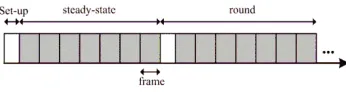
The life cycle of LEACH is divided into rounds with two phases in each round [18]. The round starts with set-up phase. It is the phase where the clusters for the current round are formed. By the end of this phase, each cluster contains a cluster-head, members, and transmission schedule. The second phase is called the steady-state. In the latter phase, the data get transferred across the network. The network continues to change from one phase to the second until it runs out of energy.
The set-up phase starts with a node contest for cluster-heads of the current round. Every eligible node participates in the self-election process by generating a random number between 0 and 1. Then, the generated number is compared with a threshold value ; if the random number is less than a threshold value, the node gets elected as a cluster-head. The threshold is set as:
= ∗ ∈
0 ℎ (1)
Where is the desired percentage of cluster-heads in each round, is the current round, and is a set of all eligible nodes that participate in the election. The set contains all the nodes who have not became a cluster-heads in the last 1/ rounds. The set members reset every 1/ rounds to contain all alive nodes. At the first round of any 1/ rounds, all nodes start with the same probability to be a cluster-head. Moreover, at the last round of the current 1/ rounds equals 1; therefore, all remaining nodes in will be elected as cluster-heads.
Figure 1. LEACH operation timeline for two rounds.
Once a node becomes a cluster-head it informs other nodes about its new status. The elected cluster-heads broadcast an advertisement message to the entire network, and then they keep their receivers on. At the same time, all non-cluster-head nodes keep their receivers on to receive the advertisement messages. These messages identify the available clusters in current round.
Upon receiving all cluster-heads’ advertisements, non-cluster nodes select the closest cluster-head and request to join it. Every non-cluster-head node compares the received signal strength of each collected advertisement and selects the highest as the nearest cluster-head. After that, the node sends a join request to the selected cluster-head, and keeps its receivers on while waiting for a
confirmation from the cluster-head. At this stage, all cluster-heads keep gathering join requests from surrounding nodes.
Each cluster-head considers the received join requests then it generates and distributes a TDMA schedule. The cluster-heads generates a TDMA schedule including all join requesting nodes; the schedule indicates the cluster-members' access time. Then the schedule is sent to all cluster-members. By receiving the TDMA schedules the cluster membership has been confirmed, and the cluster has been formed. This indicates the end of set-up phase and beginning of steady-state phase.
In the steady-state phase, the sensed data are transferred to the sink according to the cluster TDMA schedule. This phase is divided into frames. Each cluster-member has at most a single time slot in each frame. Each member keeps the transceiver off until its time slot. Each node sends the collected data in its designated time to the cluster-head. The cluster-head aggregates all received data into one message and send it to the sink. This procedure continues during the steady-state.
The steady-state phase lasts for a predefined period of time before the start of new election round. When the predefined time has elapsed, all clusters get dissociated. The status of all network nodes resets to a normal node. This way, they become ready to participate in the next election. This concludes a single round.
The duration of steady-state is set to be longer than the duration of set-up phase. The reason behind that is that the energy consumption the in set-up phase, according to the type of exchanged messaging, is higher than in steady-state. Therefore, by having a longer steady-state phase the overhead on the network is reduced.
3. Methods
To conduct this study a WSN network is simulated and run under different representative scenarios. The network uses LEACH as the network protocol. The simulations are performed using MATLAB. The network is deployed in an
MxM size grid layout. The sensor nodes are placed at the
grid points, and the sink is located at a grid corner point. The separation between a node and each of its right, left, front, and back neighbors is 10 meters. The WSN network is simulated in seven scenarios with different settings, and the performance of each situation is measured and discussed.
which is the consumption of network energy during the network operation. The aimed studies and scenarios are discussed below.
Scalability study: This study shows the effect of scaling up the network size on the performance. Three scenarios are conducted. The studies vary only in network grid size. The simulated scenarios are of networks having dimensions of 10x10, 15x15, and 20x20. The number of nodes is different in each scenario. Furthermore, they differ in the furthest distance within the network.
Multi-sink study: This study shows the effect of introducing multiple sinks on the network performance. This study compares two scenarios, a single-sink scenario and a four-sink scenario. These two scenarios are performed same size grid. The first scenario has one sink located at one corner. The second scenario has four sinks located at the grid’s four corners.
Fault tolerance study: this study shows the response of LEACH network to a failure of a group of nodes at once. There are three scenarios in this study. The network is of M equal to 10 and it has a single sink. A mass failure of random nodes is set to occur in round 265, where most of the nodes are alive and each node served as cluster-head around 13 times. However, the difference between the three scenarios is the amount of the failing nodes. The failure percentage is set as 10%, 20%, and 30% for the three scenarios.
4. Results
4.1. Scalability
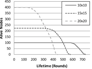
Simulating LEACH at three different scales showed a noticeable change in the network lifetime. The larger the network was the more dramatic energy dissipation, and the shorter lifetime and higher death rate it had.
Figure 2. Network Lifetime - Scalability Study.
The lifetime of the scalability scenarios is shown in Figure 2. The 10x10 scenario’s first death was in round 557, and the total round was 711. On the other hand, in the 15x15 scenario, the first death was in round 308 while the network took 567 rounds until all nodes died. Moreover, in the last scenario, the 20x20, the rounds 146 and 436 had the first death and total nodes death respectively.
Figure 3. First Death and Total Rounds - Scalability Study.
The percentage between the total rounds to the first death grows with the increase of the network grid size, as shown in Figure 3. The nodes last in the first scenario for 28% after the first death. Where, they last for 84% in the second scenario, and 199% in the 20x20 scenario.
Figure 4. Network Residual Energy - Scalability Study.
The amount of the dissipated energy, as shown in Figure 4, is proportional to the networks size. The residual energy in the 10x10 scenario decreased from 50 Joules with a slope of 0.078 ! " #$ . On the other hand, the 15x15 scenario network energy decreased with a slope of 0.236 ! " #$ . Furthermore, the third scenario slope was 0.639 ! " #$ which was the sharpest among the three scenarios.
4.2. Multi-Sink
Introducing multiple sinks to the network showed an effect on the network lifetime. The two simulated scenarios, the single-sink and the four-sink, showed that the latter scenario took longer time for the first node death.
The networks' lifetimes of the two scenarios are plotted in Figure 5. The 20x20 in size network with a single sink lasted for 146 rounds before the first node dies. On the other hand, the first death in the four-sink scenario takes place on round 357. In the four-sink scenario, after the late first death, the network has a higher death rate than in single-sink scenario. The two scenarios kept losing nodes, with higher amount of alive nodes in the four-sink scenario, until round 389 where the number of alive nodes got equal. This equivalence come after 93% of the network total rounds elapsed and energy of 72% of the nodes is drained. From this point and on, the number of operative nodes in the four-sink scenario becomes less than what it is in the single-sink scenario. After that, in the single-sink network, the last node death is on round 436, while in the four-sink case round 400 has the lost of the last node. Between the two scenarios, the nodes in the four-sink scenario last longer for the most of the network lifetime; however, the simulation results showed no significant difference in the total rounds.
Figure 6. First Death and Total Rounds - Multi-sink Study.
Figure 6 shows that there is a significant difference between the two scenarios in rounds elapsed before the first death occurred. The first death in the four-sink scenario lasted around 144% rounds more than in the single-sink scenario. Moreover, from the figure, it is noticeable that the network with four sinks has lower first death to total rounds ratio than in the single sink network. Where, in the four sinks case, the nodes last 12% more rounds after the first death. However, the remaining nodes last for 199% more rounds in the single-sink case.
Figure 7. Network Residual Energy - Multi-sink Study.
The network residual energy during the lifetime for both multi-sink study scenarios is shown in Figure 7. The energy in the four-sink network was decreasing steadily. However, with a single sink, the network dissipates more energy until 75% of the network lifetime has passed, where the energy decrement rate slows down. And, the amount of residual energy between the two scenarios got closer towards the end.
4.3. Fault Tolerance
To study LEACH toleration for nodes failure, the simulation has been conducted under three scenarios. The networks in the three fault tolerance scenarios have been set similarly except the amount of nodes loss each network experience. The effect of the different losses is described below.
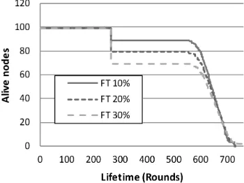
The effect of sudden deaths on LEACH is illustrated on Figure 8. In round 265, each scenario lost different amount of nodes. In the 10%, 20%, and 30% scenarios, the number of alive nodes dropped to 89, 79 and 69 respectively. The death rate, after the pre-set nodes failure, differed between the scenarios; the scenario with the least remaining nodes had the least death rate, and vice versa. However, the numbers of alive nodes in the three scenarios intersect after 95% of the total rounds has elapsed; which was in round 684. The total rounds in the three scenarios are relatively close, they are around 718 rounds. Therefore, the death of a different amount of nodes in LEACH network did not affect the total number of rounds significantly.
Figure 8. Network Lifetime - Fault Tolerance Study.
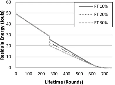
decrement slope with 0.065 ! " #$ . On the other hand, the second scenario experienced an energy decrease by 0.058 ! " #$ . The decrement slope was 0.05 ! " #$ in the last scenario, which is the least within the three scenarios. The amount of the residual energy of the three scenarios intercepted at round 370, which is after 85% of the network lifetime had been elapsed. Then, the network remaining energy did not differ much until it all drained.
Figure 9. Network Residual Energy - Fault Tolerance Study.
5. Discussion
The simulation results from section 4 reveal and confirm several aspects of LEACH protocol. Increasing the grid network size has a dramatic effect on the network lifetime. Moreover, adding multiple sinks had a positive improvement on the network lifetime. Furthermore, LEACH networks maintain its operation after nodes a mass failure.
5.1. Scalability
While examining the scalability of LEACH, it appears that larger networks suffer a higher load and has a shorter lifetime. Enlarging the network shortens the rounds elapsed before the death of both the first and the last nodes. Furthermore, the energy consumption rate in the larger networks is higher than in the smaller networks. There are two reasons behind the network lifetime shortening. First reason, larger networks cover a wider area and has longer communication distance to the sink. Therefore, the furthest cluster-heads dissipate more power to reach the sink. Second reason, bigger networks have more nodes included, which leads to a greater number of cluster-heads per round. The most burden in each round is taken by the cluster-heads, where they manage the cluster, collect the data, and send the data to the sink, which is usually further than communication distances within the cluster. As a result, by having more cluster-heads a higher amount of energy is dissipated.
Furthermore, from the study, it appears that smaller network grid size spends most of its lifetime with all nodes alive. On the other hand, in large grid network most of the
network lifetime is spent with fewer nodes than the initial amount. There are two reasons for this behavior. The first reason is the large energy consumption by far cluster-heads. They have to send data over longer distances. Thus, the far nodes consume their energy quickly, thereby, die early. The second reason is that nodes that are close to sink have better energy consumption balance. Therefore, with the time, the network loses edge nodes while the nodes close to the sink have sufficient residual energy, and this lets the network to have early node death and to then have a lower percentage of lost nodes per round. On the other hand, smaller network has better energy dissipation balance across the nodes. Consequently, the residual energy on all nodes is relatively close to each other. Therefore, once a node drained all of its energy, the remaining nodes will be at a low level of energy. That seems to be the reason for smaller network having a
higher death rate after the first death.
5.2. Multi-Sink
Having four sinks at the corner of the network increases the rounds before the first node to die. The four-sink scenario does more than twice the number of rounds than single-sink scenario before losing the first node. Introducing multiple sinks divided the network into four smaller networks. Therefore, the furthest distance to sink is decreased, that will reduce the load on the cluster-heads. On the other hand, it appears the death rate at the four-sink is higher than the rate in single-sink scenario. This is because of the average remaining energy in the nodes, at the time of the first death with four sinks, is low. In contrast, in the single-sink scenario, the first death happens earlier because of the distance to the sink with a high average of residual energy. Thus, the four-sink network nodes have higher probability to die. This observation supports the energy balance distribution provided by LEACH in the scalability study. The four-sink network lasts more with a higher number of alive nodes covering the target area.
5.3. Fault Tolerance
6. Conclusion
A better understanding of WSN protocols and their behavior is crucial. It guides to improve those protocols and to select one for certain application. The aim of the paper is to evaluate LEACH protocol under different scenarios to have a deeper understanding of that protocol. This protocol shows to provide good energy balancing within a certain range from the sinks. Load balancing appears in the three conducted studies. Furthermore, the study shows that distance between nodes and the sink has a negative effect over the network lifetime, especially in large networks. This is because that cluster-heads send data packets to sinks via single hop connection. Moreover, the three conducted studies illustrate the behavior of LEACH networks in each scenario. For future work, various protocols can be evaluated on the basis of the same benchmark scenarios. This would allow for a meaningful comparison between them.
References
[1] W. Dargie and C. Poellabauer, Fundamentals of Wireless
Sensor Networks : Theory and Practice. Chichester, West
Sussex, U.K. : Wiley, 2010.
[2] I. F. Akyildiz and M. C. Vuran, Wireless sensor networks, 1 ed. Chichester, West Sussex, U.K.: Wiley, 2010.
[3] I. F. Akyildiz, W. Su, Y. Sankarasubramaniam, and E. Cayirci, "A Survey on Sensor Networks," IEEE Communications
Magazine, vol. 40, pp. 102-114, 2002.
[4] C. F. García-Hernández, P. H. Ibargüengoytia-González, J. García-Hernández, and J. A. Pérez-Díaz, "Wireless Sensor Networks and Applications: a Survey," International Journal
of Computer Science and Network Security (IJCSNS), vol. 7,
p. 10, 2007.
[5] M. Srivastava, R. Muntz, and M. Potkonjak, "Smart kindergarten: sensor-based wireless networks for smart developmental problem-solving environments," in
Proceedings of the 7th annual international conference on Mobile computing and networking, Rome, Italy, 2001, pp.
132-138.
[6] A. Mainwaring, D. Culler, J. Polastre, R. Szewczyk, and J. Anderson, "Wireless sensor networks for habitat monitoring," presented at the Proceedings of the 1st ACM international workshop on Wireless sensor networks and applications, Atlanta, GA, 2002.
[7] K. Martinez, R. Ong, J. K. Hart, and J. Stefanov, "Glacsweb: A sensor web for glaciers," in Proceedings of European
Workshop on Wireless Sensor Networks, Berlin, Germany,
2004, pp. 46-49.
[8] F. Huang and T. Sung, "Design and Implementation of Radiation Dose Monitoring System Based on Wireless Sensor Network," in International Conference on Future
Information Technology (IPCSIT), Singapore, 2011, pp.
430-434.
[9] M. Garcia, A. Catalá, J. Lloret, and J. J. Rodrigues, "A wireless sensor network for soccer team monitoring," in 2011
IEEE International Conference on Distributed Computing in Sensor Systems and Workshops (DCOSS), Casa Convalescència, Barcelona, Spain, 2011, pp. 1-6.
[10] I. F. Akyildiz, W. Su, Y. Sankarasubramaniam, and E. Cayirci, "Wireless Sensor Networks: A Survey," Computer Networks, vol. 38, pp. 393-422, 2002.
[11] J. N. Al-Karaki and A. E. Kamal, "Routing Techniques in Wireless Sensor Networks: A Survey," IEEE Wireless
Communications, vol. 11, pp. 6-28, 2004.
[12] W. R. Heinzelman, J. Kulik, and H. Balakrishnan, "Adaptive protocols for information dissemination in wireless sensor networks," in Proceedings of the 5th annual ACM/IEEE
international conference on Mobile computing and networking, Seattle, WA, 1999, pp. 174-185.
[13] D. Peng and Q. Zhang, "An energy efficient cluster-routing protocol for wireless sensor networks," in 2010 International
Conference on Computer Design and Applications (ICCDA),
Qinhuangdao, China, 2010, pp. 530-533.
[14] S. Lindsey and C. S. Raghavendra, "PEGASIS: Power-efficient gathering in sensor information systems," in
2002 IEEE Aerospace Conference Proceedings, Big Sky, MT,
2002, pp. 3-1125.
[15] A. A. Ahmed, H. Shi, and Y. Shang, "A Survey on Network Protocols for Wireless Sensor Networks," in Proceedings of
the International Conference on Information Technology: Research and Education, Neward, NJ, 2003, pp. 301-305.
[16] K. Akkaya and M. Younis, "A Survey on Routing Protocols for Wireless Sensor Networks," Ad Hoc Networks, vol. 3, pp. 325-249, 2005.
[17] D. Bhattacharyya, T.-h. Kim, and S. Pal, "A Comparative Study of Wireless Sensor Networks and Their routing Protocols," Sensors, vol. 10, pp. 10506-10523, 2010.
[18] W. R. Heinzelman, A. Chandrakasan, and H. Balakrishnan, "Energy-Efficient Communication Protocol for Wireless Microsensor Networks," in IEEE Proceedings of the 33rd
Annual Hawaii International Conference on System Sciences (HICSS), Maui, HI, 2000, pp. 1-10.
[19] F. Xiangning and S. Yulin, "Improvement on LEACH Protocol of Wireless Sensor Network," presented at the 2007 International Conference on Sensor Technologies and Applications, Valencia, Spain, 2007.
[20] L.-Q. Guo, Y. Xie, C.-H. Yang, and Z.-W. Jing, "Improvement on LEACH by combining Adaptive Cluster Head Election and Two-hop transmission," in 2010
International Conference on Machine Learning and Cybernetics (ICMLC), Qingado, China, 2010, pp. 1678-1683.
[21] N. Kumar and J. Kaur, "Improved LEACH Protocol for Wireless Sensor Networks," in the 7th International
Conference on Wireless Communications, Networking and Mobile Computing (WiCOM), Wuhan, China, 2011, pp. 1-5.
[22] S. H. Gajjar, K. S. Dasgupta, S. N. Pradhan, and K. M. Vala, "Lifetime improvement of LEACH protocol for Wireless Sensor Network," in 2012 Nirma University International
Conference on Engineering (NUiCONE), Ahmedabad,
[23] M. Tong and M. Tang, "LEACH-B: An Improved LEACH Protocol for Wireless Sensor Network," presented at the the 6th International Conference on Wireless Communications Networking and Mobile Computing (WiCOM), Chengdu
City, China, 2010.
[24] M. F. Abad and M. A. Jamali, "Modify LEACH Algorithm for Wireless Sensor Network," International Journal of