Numerical Experiment with the Construction of a Control Operator Applied in ECGM Algorithm

Published online January 19, 2015 (http://www.sciencepublishinggroup.com/j/ajam) doi: 10.11648/j.ajam.20150301.13

ISSN: 2330-0043 (Print); ISSN: 2330-006X (Online)

Numerical experiment with the construction of a control

operator applied in ECGM algorithm

Felix Makanjuola Aderibigbe, Bosede Ojo, Kayode James Adebayo

Department of Mathematical Sciences, Ekiti State University, Ado Ekiti, Nigeria

Email address:

[email protected] (F. M. Aderibigbe), [email protected] (B. Ojo), [email protected] (K. J. Adebayo)

To cite this article:

Felix Makanjuola Aderibigbe, Bosede Ojo, Kayode James Adebayo. Numerical Experiment with the Construction of a Control Operator Applied in ECGM Algorithm. American Journal of Applied Mathematics. Vol. 3, No. 1, 2015, pp. 8-13. doi: 10.11648/j.ajam.20150301.13

Abstract:

In this paper, we constructed a control operator, G, which enables an Extended Conjugate Gradient Method (ECGM) to be employed in solving for the optimal control and trajectories of continuous time linear regulator problems. Similar operators constructed in the past by various authors have limited application. This call for the construction of the control operator that is aimed at taking care of any of the Mayer’s, Lagrange’s and Bolza’s cost form of linear regulator problems. The authors of this paper desire that, with the construction of the operator, one will circumvent the difficulties undergone using the classical methods and its application will further improve the result of the Extended Conjugate Gradient Method in solving this class of optimal control problem. The constructed Linear Control Operator is applied in ECGM algorithm to solve Continuous-Time Linear Regulator Problems with the convergence profile showing the efficiency of the operator.

Keywords:

Continuous Linear Regulator Problem, Control Operator, Extended Conjugate Gradient Method, Optimal Control

1. Introduction

Consider the linear regulator problem of the Bolza type in [1] and [6] as:

Problem (1):

, , . = 1₂

+ + (1.1)

subject to the differential state equation

= ! + " , 0 ≤ ≤ , (1.2)

where H and are real symmetric positive semi-definite % × % matries. is a real symmetric positive definite ' × ' matrix, the initial time, and the final time, , are specified. is an n-dimensional state vector, is the m-dimensional plant control input vector. (% are not constrained by any boundaries. ! (% " are specified constants which are not necessarily positive. For H = 0, (1.1) is called a Lagrange problem, but if Q(t) = R(t) = 0, it is called a Mayer problem.

The form (1.1) may be rewritten as:

= ) * +1₂

+ + (1.3)

= + +

(1.4)

= . + +

/ .

As customary with penalty function techniques, constrained problem equations (1.2) and (1.4) may be put into the following equivalent form:

〈1, 21 〉4 = '5%6,7 +

+

(1.5)

where 8 > 0 is the penalty parameter and ‖ − ! − " ‖ is the penalty term.

Let us denote by <= the product space

<= = ℋ?0, @ × ℓ ?0, @ (1.6)

is the product space of Sobolev space ℋ?0, @ of absolutely continuous function . such that, both . (% . are square integrable over the finite interval [0, ] and the Hilbert space ℓ CD, E] of equivalence classes of real valued functions on [D, E] with norm defined by:

‖F . ‖ℓGCH,I]= |F |

I H

K G

, F . L ℓ CD, E] (1.7)

Then, the inner product〈. , . 〉₄₌on <= is given by

〈. , . 〉4= = 〈. , . 〉ℋ? , @+ 〈. , . 〉ℓG? , @ (1.8)

Suppose 1( ) ∈ <= denotes the ordered pair

1 ( ) = ( ), ( ) ; ( ) ∈ ℋ?0, @, ( ) ∈ ℓ ?0, @ (1.9)

then, we seek to determine the operator G on <= such that

〈1, O1 〉_<== {₀F P( ) ( )+1₂ P( ) ( ) ( )+

1 2

P

( ) ( ) ( )

(1.10)

+ 8‖ ( ) − !( ) ( ) − "( ) ( )‖ }

where <= is suitably chosen Hilbert space. The control operator, G, is then utilized in the iterative framework of the CGM in order to arrive at a solution of problem (P1). We provide a recapitulation of the formal CGM in the next section for the sake of completeness.

2. Conjugate Gradient Method

Algorithm

The Conjugate Gradient Method (CGM) algorithm for iteratively locating the minimum ∗ of F( ) in ℋ as described by [4] is as follows:

Step 1: Guess the first element ϵ ℋ and compute the remaining members of the sequence with the aid of the formulae in the steps 2 through 6.

Step 2: Compute the descent direction R = −S (2.1a)

Step 3: Set _{TU V T}+ D_TR_T ; where D_T= _〈Y〈WX,WX〉ℋ

X,ZYX〉ℋ (2.1b) Step 4: Compute S_TU = S_T + D_T2R_T (2.1c)

Step 5: Set R_TU = −S_TU + E_TR_T ; E_T= 〈WX[K,_〈W WX[K〉ℋ

X, WX〉ℋ (2.1d) Step 6: If S_T = 0 for some i, then, terminate the sequence; else set i = i + 1 and go to step 3.

In the iterative steps 2 through 6 above, R_T denotes the descent direction at i-th step of the algorithm, D_T, is the step

length of the descent sequence { _T} and S_T denotes the gradient of F at _T. Steps 3, 4 and 5 of the algorithm reveal the crucial role of the linear operator G in determining the step length of the descent sequence and also in generating a conjugate direction of search. Applicability of the algorithm thus depends solely on the explicit knowledge of the operator G. Generally, for discrete optimization problems, G is readily determined (see [4, pp. 51-53]); and such problem enjoys the beauty of the CGM as a computational scheme since the CGM exhibits quadratic convergence and requires only a little more computation per iteration. [2] opined that these properties make the CGM a fascinating computational technique with a strong appeal for implementation on the digital computer.

However, for the type of constrained continuous linear time regulator problem (P1) discussed in this paper, application of the CGM algorithm as presented is hindered because then, the equivalent of operator G which satisfies (P1) in this sense of (1.13) is not readily found and construction of such operator is the main aim of this paper. The construction of such an operator is not new. For instance in [5], the authors constructed the control operator for the following related problem respectively as:

Problem (2)

\5%(6,7) _^{( ( ) + ] ( )} (2.2)

Subject to

( ) = _ ( ) + ( ), ≤ ≤ , (2.3)

( ) = ; (2.4) where a, b, c and d specified constants such that a>0, b>0; _, are given, ( ) denotes the derivative of the state (. ) with respect to time, and (. ) is the control vector. The resulting control operator G is of the form:

(2 )( ) = −8C (0) − ` (0)]a5%ℎ( ) + 8 C (c) − ` (c)]`dcℎ( − c) c

(2.5)

− C(! + 8` ) (c) − 8` (c)] a5%ℎ( − c) c

+C(( + 8` ) (0) − 8` (0)]`dcℎ( )

+_{eTfg( )}eTfg( ){(( + 8` ) (P) − 8` (P) + 8a5%ℎ(P)C (0) − ` (0)]

− 8 C (c) − ` (c)]`dcℎ (P − c) c

+ C(! + 8` ) (c) − 8` (c)] a5%ℎ(P − c) c

− C(! + 8` ) (0) − 8` (0)]`dcℎ(P)}, 0≤ ≤ P

(2 )( ) = 8h (0)a5%ℎ( ) − 8 h (c)`dcℎ( − c) c

(2.7)

+8 `h (c)a5%ℎ( − c) c + 8`h (0)`dcℎ( )

+_{eTfg( )}eTfg( ){8`h (P) − 8h (0)a5%ℎ(P)

+8 h (c)`dcℎ(P − c) c + 8 `h (c)a5%ℎ(P − c) c

+ 8`h (0)`dcℎ(P)}, 0≤ ≤ P

(2 )( ) = " ( ) + 8h ( ), 0≤ ≤ P (2.8) Based on 2.5 – 2.8 above, one can obtain the desired 2R_Tto apply 2.1c which would henceforth allow us to exploit the simplicity of the conjugate gradient method algorithm.

Similarly, Aderibigbe, (1993), constructed a control operator for a linear regulator problem with delay parameter as:

Problem (3)

\5%(6,7) _^{! ( ) + " ( )} (2.9)

Subject to

( ) = ` ( ) + ` ( − i) + h ( ), ≤ ≤ , (2.10)

( ) = ℎ( ); −i ≤ ≤ 0 (2.11) where !, " > 0; the delay parameter i > 0 and are given; ` , ` (% h are specified constants which are not necessarily positive and ℎ( ) is a given piecewise continuous function which is of exponential order on C−i, 0]. For detail, see [2].

3. Main Result

Our results for problem (P1) are contained in the following theorem:

3.1. Theorem 1

Let us denote by < j the product space

<= = k , _{? , @ × ℓ ? , @ (3.1)}

of the Sobolev space of absolutely continuous function (. ) on [ , ] and the usual Hilbert space ℓ ? , @ of Lebesgue measurable, real-valued functions which are square integrable on the closed interval , ]. Then ,for 8 > 0 there exists a control operator, G, with 2: <= × < j → ℛ such that

〈1 , G1 〉4= = _^ + +

+ 8‖ ! + " − ‖ (3.2)

where 1 = , . Furthermore, G is explicitly given by

G1 ≡ qG_G G_{G r = q} 2₂ + 2_{+ 2} r (3.3)

where the composite operators 2_Ts, 1 ≤ 5, t ≤ 2 are given as follows:

2 = −8 0 a5%ℎ + 8 c `dcℎ − c − a5%ℎ − c

(3.4)

× u + 8! c + − 28! c v c + u + 8! 0 + − 28! 0 v

× `dcℎ +_eTfg eTfg + 8! + − 28! − C + 8! 0

+ − 28! 0 ]`dcℎ + 8 0 a5%ℎ − 8 c `dcℎ − c c

+ a5%ℎ − c C + 8! c + − 28! c ] c ; 0 ≥ ≥

2 =

28!" 0 `dcℎ − 28!" c a5%ℎ − c c +

eTfg

eTfg 28!" _(3.5)

−28!" 0 `dcℎ + 28!" c a5%ℎ − c c ; 0 ≥ ≥

2 = −28" ; 0 ≥ ≥ (3.6)

2 = q1_{2 + 8" r} ; 0 ≥ ≥ (3.7)

Proof of Theorem 3.1

In an attempt to proof the above theorem, we need the following fundamentals:

3.2. Lemma 1

Let % ≥ 0 be an integer and suppose `f 0, P denotes the space of all real-valued functions x , 0 ≤ ≤ P which are n-times continuously differentiable on C0, P] ⊂ ℛ with the norm ‖x‖_fgiven by

‖x‖f= ∑ '(fTV { { |xT |, (3.8)

differentiable and _•• E( ) = D( ) for all ∈ C(, ]]. Proof

For our subsequent development we shall associate with the right hand side of (1.10) the functional _€(1 ,

1 ) defined by

€(1 , 1 ) = { ( ) ( ) + ( ) ( ) +

( ) ( ) + 8 ( ) ( )

(3.9)

−8! ( ) ( ) − 8" ( ) ( ) − 8! ( ) ( ) + 8! ( ) ( )

+8!" ( ) ( ) − 8" ( ) ( ) + 8!" ( ) ( ) + 8" ( ) ( )}

where 1 = ( ), ( ) , 1 = ( ), ( ) are the ordered triple pair which belong to the space <= defined by (3.1). It follows that; the form (3.9) is equivalent to (3.2) under the equivalent relationships:

• _{( ) ≡ ( ) = ( ), 0 ≥ ≥ ,}( ) ≡ ( ) = ( ), 0 ≥ ≥ , ( ) ≡ ( ) = ( ), 0 ≥ ≥ .‚

(3.10)

For proof, see [7]. We then have the following proposition:

3.3. Proposition 1

€(1 , 1 ) is a bounded, bilinear, self-adjoint form on <=. Proof:

Bilinearity and self-adjointness of _€(1 , 1 ) is clear from its definition; and its boundedness follows from the fact that 1_T( ) = _T( ), _T( ) , 5 = 1, 2 is bounded.

3.4. Remarks

By virtue of proposition above and a consequence of the Reiess representation theorem on Hilbert spaces [8], it follows that _€(1 , 1 ) induces a uniquely determined, bounded linear operator G say on <= with the representation

€(1 , 1 ) = 〈21 , 1 〉4== 〈1 , 21 〉4= = €(1 , 1 ) (3.11)

where it is clear that G is also self-adjoint on <= since _€(1 , 1 ) is.

Let us now consider the equivalence

〈1 , 21 〉 = 8〈1 , 1 〉 (3.12)

This is convenient for our subsequent developments. Then, let 1 ( ) = ( ), ( ) , then we can write

(G1 (t)) ≡ qG G

G G r q ( )( )r = q(2 )( ) + (2 )( )r (2 )( ) + (2 )( ) (3.13)

On setting ( ) = 0; then (3.14) will implies

(G1 (t)) ≡ q(2 )( )

(2 )( )r = qx ( )x ( )r (3.14)

where the functions x ( )(% x ( ) must be determined in order to know (2 )( )(% (2 )( ). By virtue of the equivalence (3.10), we set ( ) = 0, in (3.9) as:

〈1 ( ), 1 ( )〉 = { ( ) ( ) + ( ) ( ) +

8 ( ) ( ) − 8! ( ) ( ) − 8" ( ) ( ) − 8! ( ) ( ) + 8! ( ) ( ) − 8" ( ) ( )} (3.15)

On simplifying (3.15) further, we obtain

〈1 ( ),1 ( )〉 = { ( )C( + 8! ) ( ) + ( − 28!) ( )] + ( )C8 ( )] (3.16)

〈1 ( ),1 ( )〉 = { ( )x ( ) + ( )x ( ) + ( )x ( )} (3.17)

The quantities x ( ) (% x ( ) which satisfy (3.17) have to be determined. Towards this, we set

D( ) = ( + 8! ) ( ) + ( − 28!) ( ) (3.18)

E( ) = 8 ( ) (3.19)

where E( ) is the derivative of D( ) from (3.16) and D( ) = x ( ) while E( ) = x ( ) then, D( ) −

x ( ) (% E( ) − x ( ) are continuous functions on C0, ] and for (. ) ∈ 2 C0, ] such that (0) = 0 =

( ), we have

{ ( )C D( ) − x ( )] + ( )CE( ) − x ( )]} = 0,(3.20)

so that by Lemma 1, E( ) − x ( ) is differentiable on C0, ] with

•

• CE( ) − x ( )] = D( ) − x ( ). (3.21)

This implies that

xƒ ( ) − x ( ) = E ( ) − D( ) (3.22)

Using (3.18) and (3.19) in (3.22), we obtain

xƒ ( ) − x ( ) = 8 ƒ ( ) − C + 8! ( )

+( − 28!) ( )] (3.23)

Now from (3.17), we obtain

( )x ( ) = ( )C−28" ( )] (3.24) From which we obtain by virtue of (3.14)

x ( ) = (2 )( ) = −28" ( ); 0 ≤ ≤ (3.25) To determine x ( ), the second order differential equation (3.23) must be solved. For this purpose, let

F( ) = 8 ƒ ( ) − C + 8! ( ) + ( − 28!) ( )] (3.26) Then, (3.23) takes the form

xƒ ( ) − x ( ) = F( ); 0 ≤ ≤ (3.27)

the initial conditions

x (0) = % (% x (0) = ' (3.28)

where the quantities % (% ' need to be determined. In view of this, let „(c) = ℒ{F( )} and

x (c) = ℒ{x ( )} denote the Laplace transforms of F( ) and x ( ) respectively, then by taking the Laplace transform of (3.27) and (3.28), we get

c x (c) − x (c) − % c − ' = „(c) (3.29)

We proceed to determine the

quantities x ( ), % (% ' appearing in (3.29) solving (3.29) and the resulting constants therein eliminated, we obtain the following tidier form:

x ( ) = −8 (0)a5%ℎ + 8 (c)`dcℎ − c − a5%ℎ − c × u + 8! (c) + ( − 28!) (c)v c

+ u + 8! (0) + ( − 28!) (0)v × `dcℎ

+_eTfg eTfg { + 8! + ( − 28!)

−C + 8! (0) + ( − 28!) (0)]`dcℎ + 8 (0)a5%ℎ

− 8 (c)`dcℎ − c c

+ a5%ℎ − c C + 8! (c) + ( − 28!) (c)] c} ;

0 ≥ ≥ (3.30)

Thus, the first column of the operator, 2 (% 2 are uniquely determined by virtue of (3.30) and (3.25) respectively.

Repeating the same arguments, we obtain the second column of the operator, 2 (% 2 , by setting ( ) = 0 in (3.9) from which we obtain

x ( ) = 28!" (0)`dcℎ − 28!" (c)a5%ℎ − c c

+_{a5%ℎ †28!" (}a5%ℎ − 28!" (0)`dcℎ

+ 28!" (c)a5%ℎ − c c} ; 0 ≥ ≥ (3.31)

x ( ) = + 8" ( ); 0 ≥ ≥ (3.32)

This concludes the proof of Theorem 3.1.

4. Implementation of the Constructed

Operator in ECGM Algorithm

The following linear regulator problems were solved using the ECGM algorithm described above.

Problem (P1):

( , , (. )) = (1) + { ( ) + ( )}

subject to

( ) = 2 ( ) + 3 ( ), 0 ≤ ≤ , = 5 (% = 3

Problem (P2):

( , , (. )) = (1) + { ( ) + ( )}

subject to

( ) = −3 ( ) − 2 ( ), 0 ≤ ≤ , = 5 (% = 3

Problem (P3):

( , , (. )) = (1) + { ( ) + ( )}

subject to

( ) = 5 ( ) + 3 ( ), 0 ≤ ≤ , = 2 (% = 3

5. Conclusion

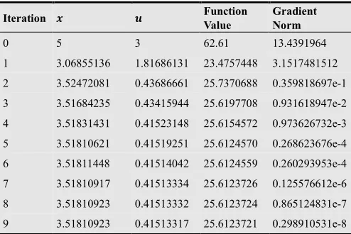
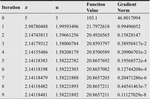
It follows from here that, while [5] constructed an operator for CLRP, [2] focuses on same class of optimal control problem but with delay parameter in the state variable. The construction of this control operator, G, helps to bridge the gap between Bolza form of CLRP and Lagrange as well as Mayer Forms of CLRP. This makes the construction of the operator very important and relevant in that, it takes cares of the variations in CLRP with or without boundary penalty variable. In determining the convergence of the problems under review, the Gradient Norm was used and set at 10‰ and the Function Value was also considered at the point when the function value starts to repeat itself. From the Tables 1 and 2, Problems (P1) and (P2) converged at the 9th iteration with gradient norms 2.98910531e-9 and 1.1127029e-9 respectively while problem (P3) converged at the 23rd iteration with gradient norm 3.5220424e-9.

Table 1. Table of Result (P1): At Penalty Parameter 8 = 0.01

Iteration Š ‹ Function

Value

Gradient Norm

0 5 3 62.61 13.4391964

1 3.06855136 1.81686131 23.4757448 3.1517481512

2 3.52472081 0.43686661 25.7370688 0.359818697e-1

3 3.51684235 0.43415944 25.6197708 0.931618947e-2

4 3.51831431 0.41523148 25.6154572 0.973626732e-3

5 3.51810621 0.41519251 25.6124570 0.268623676e-4

6 3.51811448 0.41514042 25.6124559 0.260293953e-4

7 3.51810917 0.41513334 25.6123726 0.125576612e-6

8 3.51810923 0.41513332 25.6123724 0.865124831e-7

Table 2. Table of Result (P2): At Penalty Parameter 8 = 0.1

Iteration Š ‹ Function

Value

Gradient Norm

0 5 3 103.1 46.8017094

1 2.98780488 1.99593496 21.7972618 0.99496052

2 2.14743813 1.59661256 20.4926565 0.15828147

3 2.14179312 1.58006784 20.8593797 0.38950417e-2

4 2.14155486 1.58208179 20.8700589 0.20906703e-2

5 2.14118383 1.58222782 20.8657692 0.19568572e-4

6 2.14118198 1.58222303 20.8657082 0.12744208e-4

7 2.14118479 1.58221888 20.8657205 0.20471286e-6

8 2.14118482 1.58221893 20.8657211 0.44541463e-7

9 2.14118481 1.58221892 20.8657211 0.11127029e-8

Table 3. Table of Result (P3): At Penalty Parameter 8 = 0.1

Iteration Š ‹ Function

Value

Gradient Norm

0 2 3 53.1 25.8069758

1 -0.74256891 1.04102221 2.22132825 1.35523175 2 -1.53027208 2.02974998 9.04736912 1.55635029 3 -1.51972594 2.27465778 9.85321115 0.26905925 4 -1.49421917 2.28021637 9.70451487 0.12727048 5 -1.46725095 2.24614227 9.38654563 0.11204496 6 -1.46919089 2.23082279 9.33631847 0.1942723e-1 7 -1.47122794 2.23059326 9.34870783 0.10412658e-1 8 -1.47337643 2.23362683 9.37512075 0.83226081e-2 9 -1.47315285 2.23465202 9.37782731 0.14227137e-2

References

[1] Athans, M. and Falb, P. L., (1966), Optimal Control: An Introduction to the Theory and Its Applications, McGraw-Hill, New York.

[2] Aderibigbe, F. M., (1993), “An Extended Conjugate Gradient Method Algorithm for Control Systems with Delay-I”, Advances in Modeling & Analysis, C, AMSE Press, Vol. 36, No. 3, pp 51-64.

[3] George M. Siouris, (1996), An Engineering Approach To Optimal Control And Estimation Theory, John Wiley & Sons, Inc., 605 Third Avenue, New York, 10158-00 12.

[4] Hasdorff, L. (1976), Gradient optimization and Nonlinear Control. J. Wiley and Sons, New York.

[5] Ibiejugba, M. R. and Onumanyi, P., (1984), “A Control Operator and some of its Applications, J. Math. Anal. Appl. Vol. 103, No. 1. Pp. 31-47.

[6] David, G. Hull, (2003), Optimal Control Theory for Applications, Mechanical Engineering Series, Springer-Verlag, New York, Inc., 175 Fifth Avenue, New York, NY 10010. [7] Gelfand, I. M. and Fomin, S. V., (1963), Calculus of

Variations, Patience Hall, Inc., New Jersey.