Hybrid Adaptive Fuzzy Neural Network Control for Grid-Connected SOFC System

Published online December 29, 2014 (http://www.sciencepublishinggroup.com/j/ijepe) doi: 10.11648/j.ijepe.20150401.11

ISSN: 2326-957X (Print); ISSN: 2326-960X (Online)

Hybrid adaptive fuzzy neural network control for

Grid-connected SOFC system

Sadaf Sardar

1

, Amjid Ullah Khattak

1

, Shahid Qamar

2, *

1

Department of Electrical Engineering, University of Engineering and Technology, Peshawar, Pakistan 2

Department of Electronic Engineering, International Islamic University, Islamabad, Pakistan

Email address:

[email protected] (S. Sardar), [email protected] (A. U. Khattak), [email protected] (S. Qamar)

To cite this article:

Sadaf Sardar, Amjid Ullah Khattak, Shahid Qamar. Hybrid Adaptive Fuzzy Neural Network Control for Grid-Connected SOFC System.

International Journal of Energy and Power Engineering. Vol. 4, No. 1, 2015, pp. 1-10. doi: 10.11648/j.ijepe.20150401.11

Abstract:

The solid oxide fuel cell (SOFC) is widely acknowledged for clean distributed power generation use, but critical process problems frequently occur when the stand-alone fuel cell is directly linked with the electricity grid. To guarantee the optimal operation of the SOFC in a power system, it is essential, that its generation ramp rate and load following is fast enough to sustain power quality. In order to address these problems, a suitable and highly efficient control system will be required to control and track power load demands for complex SOFC power systems under grid connection. Therefore, novel nonlinear hybrid adaptive Fuzzy Neural Network (AFNN) is developed for control of grid connected SOFC. During peak power demand schedules from electric utility grid and large load perturbations, maintaining optimal power quality and load-following is a big challenge. Both the rapid power load following and safe SOFC operation requirement is taken into account in the design of the closed-loop control system. Simulation results showed that the proposed hybrid AFNN enhance the optimal power quality and load-following than conventional PI controller.

Keywords:

Neural Netwrok, Fuzzy Logic, Distributed Generation, SOFC

1. Introduction

Distributed generation (DG) is a promising technology that can be used to address some of the technical as well as environmental concerns in power systems. As a kind of high-temperature fuel cell, SOFC presents an attractive option for the DG technology because it is modular, efficient and environmentally friendly. Unlike other types of fuel cells, the SOFC is entirely solid state with no liquid components. It usually works at a high temperature, in the range of 800– 1000 ◦C to reach the electrolytes ionic conductivity requirement [1].

As one of the second generations of fuel cells, the SOFC has been demonstrated to be a promising power generation technology, especially in stationary applications [2-6]. The SOFC/gas turbine (GT) based distribution generation can provide ancillary services such as load following and regulation with respect to the current deregulation and unbundling of the energy market [5, 6]. However, load following problems occur when the response of the fuel cell system cannot safely meet both the external power load demand and the balance of parasitic plant power demand [7].

For example, the phenomenon of oxygen starvation will appear in a fuel cell when the sudden power load changes greatly [8]. In that case, the partial pressure of oxygen falls dramatically, accompanied by rapid decrease in cell voltage, which would shorten the life of the fuel cell stack. On the other hand, the fuel cell may also be permanently damaged when the fuel starvation occurs in case of deficient fuel supply [9, 10]. Therefore, an effective control system is in great demand to ensure that the fuel cell system meets the time-varying power load demand with high process operation efficiency [2-11].

examined in [16]. Also, model predictive control design for SOFC is presented in [17]. Although the control ofnonlinear SOFC system is challenging due to the slow response under tight safe operation constraints, several predictive control strategies have been proposed for rapid load following. In [18], a fuzzy Hammerstein model was identified from the input–output operation data of an SOFC stack, and then the associated standard predictive controller was applied to the fuel control of the stand-alone SOFC stack to meet stepwise power load demands. Unfortunately, the stability issues of these closed-loop model predictive control systems have been largely ignored.

Classical and intelligent control strategies have been applied to the control system of renewable energy technology [19]. Conventional control algorithms, i.e., PI controllers require precise mathematical model of the system and are very complex to parameter discrepancies [20]. Intelligent control techniques such as artificial neural networks, fuzzy logic, or neuro-fuzzy are more effective and vigorous than conventional control, since they do not require model of the system and enhance the dynamic performance of the system. Among the fuzzy neural network has faster in convergence and ability to improve dynamic behavior of the system.

Fuzzy logic models have been widely accepted in control community for its capability to represent nonlinear dynamics. Fuzzy systems are demonstrated to have very good approximation and interpretation capability to general nonlinear systems [21-23]. The transient performance is of much more concern in industrial process control and economical plant operation. Fortunately, several neuro-fuzzy based predictive control approaches have been developed most recently [24, 25]. Many researcher worked on fuzzy logic control interfacing with renewable technologies is presented in [26, 27].

As to overcome aforementioned control problems, highly nonlinear control approaches are required to meet peak power demand schedules from electric utility power and maintaining optimal power quality. Therefore, novel nonlinear hybrid adaptive Fuzzy Neural Network (AFNN) is developed for control of grid connected SOFC. In this study, AFNN control algorithm is designed to control and track power load demands for complex SOFC power systems under grid connection. Both the rapid power load following and safe SOFC operation requirement is taken into account in the design of the proposed closed-loop control system.

2. SOFC Dynamic Modeling

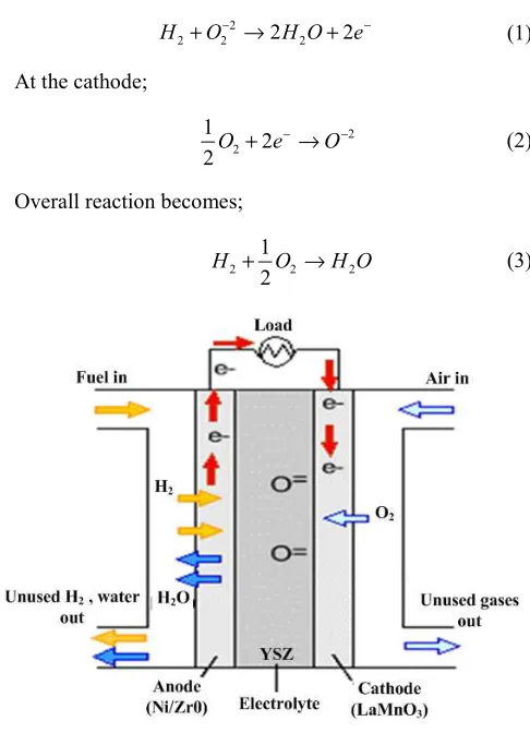
SOFC is a type of fuel cell, which operates at high temperature range of 600-1000C. The electrolyte material is a solid metal oxide ceramic, generally dense Yttrium Stabilized Zirconia (YSZ) (Y203stabilized with ZrO). YSZ proved to be very good material for the conduction of negatively charged ions, which are O2in case of SOFC. The typical structure and components of SOFC are shown in Figure 2. The fuel electrode or anode is usually made of a cement like material, a mixture of zirconium oxide (CO=ZrO2or Ni=ZrO) and

cobalt (Co) or nickel (NI). The Co or Ni gives conductivity improvement, and the whole cement mixture enhances negative ion conductivity. The air electrode or cathode is made of an ion conducting ceramic mixture [28], which is strontium-doped lanthanum magnetite (LaMnO2). At the anode, preheated hydrogen molecule is oxidized by releasing two electrons, which flow through the external circuit and feed the load. At the cathode, reduction of preheated air or oxygen molecule take place by absorbing two electrons coming from external circuit. This taking up of electrons make it negatively charged ions. Concentration gradient of oxygen occurs, which result in ion migration from cathode through the electrolyte via vacancy transport to the anode side. Equations (1) to equation (3) show the chemical reactions associated with SOFC.

At anode;

2

2 2 2 2 2

H +O− → H O+ e− (1) At the cathode;

2 2

1 2

2O e O

− −

+ → (2)

Overall reaction becomes;

2 2 2

1 2

H + O →H O (3)

Figure 1. Schematic of SOFC

• Hydrogen is supplied at the anode and oxygen at the cathode.

• Gases considered in this system are ideal.

• For output cell voltage, Nernst voltage applies.

• Stable cell temperature is considered.

• Voltage losses (ohmic, activation, concentration) are considered.

2.1. Gibb’s Free Energy Theory

In the development of fuel cell’s mathematical model, Gibb's free energy provides the basic diagnostic understanding. Gibb's free energy can be termed as the energy which performs external work. This work done is not due to variation in the volume or pressure levels of reactants and products involve in the fuel cell. In this condition, the movement of electrons in the external circuit is referred to as “external work” or electrical work done. Gibb's free energy at slandered temperature (STP) is represented by “Gs”. The

changes occur in this parameter G is critical and is related with release of free energy. Mathematically, this change is the difference between Gibb's free energies of reactants and products i.e;

products reactants

s s s

G G G

∆ = − (4)

Gibb's energy per mole can be written as;

products reactants

s s s

g g g

∆ = − (5)

In the electrochemical process of SOFC, the reactants are hydrogen and oxygen and product is water, so equation 5 can be written as

;

2 2 2

1

( ) ( ) ( )

2

s s H O s H s O

g g g g

∆ = − − (6)

The open circuit potential of SOFC can be shown as;

2 s g E F ∆

= − (7)

where, F is Faraday's constant, and its value is 96487 C/mol.

2.2. Variation in Pressure

The Gibb’s free energy and voltage of SOFC depends on variations in temperature and pressures. Equation 8 shows how the parameter ∆gschange from its standard value ∆gstp;

2 2

2

0.5

ln H O

s s

H O

P P

g g RT

P

°  

∆ = ∆ − _ _

  (8)

where, R is universal gas constant having a value of (8.314 J/mol K), T is the operating temperature and PH2, PO2 and Pare the partial pressures of hydrogen, oxygen and water respectively. The relation for fuel cell voltage at STP can be written as; 2 g E F °

°_{= −}∆ ₍₉₎

Using equations (7), (8) and (9), the “Nernst potential” E of SOFC can be representedas follows;

2 2

2

0.5

ln

2

(

)

H O N H O P P RT E E F P °

= + (10)

Nernst equation is used to relate the open circuit cell potential with varying pressure at standard temperature.

2.3. Partial Pressures Calculation

For the calculation of partial pressure of any gas, famous “ideal gas equation” is extensively used.

pv=nRT (11)

In case of SOFC, the partial pressure of hydrogen can be written using ideal gas relation as follows;

2 2 H H anode m RT P V

= (12)

where, Vanode=Volume of the anode, mH2= Number of moles

of hydrogen

Taking derivative on both sides of equation (12), getting;

2

2 2

H

H anode anode H

m R T

d d R T d

P m

dt =dt V =V dt (13)

where uh2 is the derivative of mh2, and it represents the molar

flow rates of hydrogen with units (Kmols-1). There are three quantities, which represent the overall molar flow rate of hydrogen in SOFC;

2 ( 2 2 2)

in out r

H anode H H H

d R T

P u u u

dt =V − − (14)

where

2 in H

u = Hydrogen molar flow rate in the anode channel

2 t H ou

u = Hydrogen molar flow rate out of anode channel

2 r H

u = Hydrogen molar flow rate which reacts in the

channel

Considering the electrochemical laws, the amount of hydrogen which reacts in the cell is given by;

2 ₂ 2

r FC

H p FC

N I

u K I

F

°

= = (15)

where

N = Number of cells in SOFC stack

IFC= Current provided by stack KP= Modeling constant,

Equation (15) shows that fuel cell output current is directly proportional to hydrogen molar flow rate

2. r H

u The value of

occurring at load side. Whenever current demand changes at the inverter input, that value is fed back to the reformer controller, which is responsible for changing the position of fuel valve. In this way, changes in active power are translated back by current to fuel cell for required flow of fuel in the channel. Putting the value from equation (15) in equation (14), the differential relation of hydrogen partial pressure can be written as:

2 ( 2 2 2 )

in out

H anode H H P F

d R T

P u u K I C

dt =V − − (16)

By setting the initial conditions to zero, Laplace transform operation on both sides yield;

2

2 2

2

1

( 2 )

1

H in

H H P FC

H

K

P u K I

S

τ −

= −

+ (17)

where, 2 H

τ

is the system pole value, concerned with hydrogen valve time constant,and it is expressed as;

2 2 anode H H V K R T

τ = (18)

Equation (17) represents the value of partial pressure, incorporated in Nernst equation to calculate cell voltage. In similar manner, partial pressures for oxygen and water become;

2

2 2

2

1

( 2 )

1

O in

O O P FC

O

K

P u K I

S

τ −

= −

+ (19)

2 2 2 1 (2 ) 1 H O

H O P FC

H O

K

P K I

S

τ − =

+ (20)

2.4. SOFC Temperature Calculation

Heat produced by fuel cell can be used to estimate the change in temperature of SOFC. Further, this change in temperature is used for computing the working temperature of SOFC. Total heat generated is formulated as;

(1.485 )

net FC SOFC

q =nI −V (21)

net

q T

MC

∆ = (22)

Where, M and C are the mass and specific heat energy constant of fuel cell stack, whose values are 44kg and 560J/kg-k, respectively. This change in temperature is used to determine the working temperature of the SOFC stack;

initial

T =T + ∆T (23)

2.5. Fuel Utilization

The slow response of fuel cell current can be related by equation (21); 1 ref FC e I I S τ   =  +

  (24) whereτ_eis the electrical time constant and Irefis the reference

or desired currentwhen the output power is Pref..

Mathematically;

=

ref ref SOFC

P

I

V

(25)

Equations for fuel flow in terms of its utilization are represented by equation below;

2 2 1 1 P H f K u

U τ S

 

= _ _

+

  (26)

Where τ_fis the response time of fuel and 2 H

u is the “fuel

utilization” factor. It is the ratio of fuel used in the cell to the total fuel supplied at the input. Generally, a range between 80-90% is selected for fuel utilization.

2.6. Stack Voltage Calculation

Nernst equation is generally used for the calculation of SOFC output DC voltage ESOFC. Mathematically;

2 2 2 0.5 ln 2 H O SOFC H O P P RT

E N E

F P

° °  

=  +   

    (27)

There are three types of losses occurring in fuel cell, due to which terminal cell voltage VSOFC is less than total cell

voltage.

SOFC SOFC act ohm conc

V =E −υ −υ −υ (28)

where υ υ_act, _ohm,andυ_conc , are the activation, ohmic and concentration losses.

3. SOFC-Grid Interfacing

SOFC is one of the DG technologies, which generates a DC power by an electrochemical energy conversion process. The generated DC voltages are low and variable, thus the fuel cell cannot be connected to the utility mains directly. To make this interface between SOFC and grid possible, suitable power electronic converters are used. One such integration between SOFC system and utility grid using a “power conditioning system” (PCU) is depicted in Fig. 2. The PCU consist of following components:

• DC-AC Inverter

• RL Filter

Figure 2. Grid connected SOFC system

3.1. Active Power Control

For controlling the active power of SOFC system connected to the utility grid, an equivalent circuit is shown in Fig. 3. Two voltage sources are considered connected through line inductance L. VSOFC is the fuel cell voltage, VG

represents grid side voltage and δ is the phase angle between SOFC and grid voltages.

Figure 3. Equivalent circuit of SOFC system

The complex power provided by SOFC system (neglecting VSI and transformer losses) to the utility grid is given by;

SOFC FC

S = +P jQ=V I∗ (29) In this work, reactive power is set to zero. The flow of active power from SOFC to grid is represented as follows;

sin( )

SOFC G

mV V

P

L δ

ω

= (30)

where m is the per unit value of variable modulation index. Using equations (28) to (30), current drawn from fuel cell can be shown as;

sin( )

G FC

mV I

L δ

ω

= (31)

In order to comply with active power demand and load

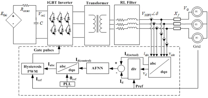
following schedules, proper controller for inverter is essential. For this purpose, an AFNN is implemented with hysteresis current PWM to provide suitable gate pulses to the inverter, so that desired output power is generated.

3.2. Inverter Topology

There are two main types of inverters on output wave form basis, i.e., “square wave” and (PWM) inverters. A square AC wave output is generated by square wave inverters which can be altered by changing the input DC voltage. On the other hand, a switching sequence is used for PWM inverters to produce an AC output waveform.

In this case study, a 3-phase inverter is considered in which switching devices are Insulated Gate Bipolar Transistors (IGBT). At the inverter input, DC voltage is provided by SOFC and followed by a DC link capacitor to filter out any pulsations in the incoming DC supply. RL filter at the output of inverter ensures the elimination of current harmonics to meet required standards. Schematic diagram of inverter topology is shown in Fig. 4.

Figure 4. IGBT inverter topology

3.3. Series Filter

A series filter circuit having inductance La and resistance Ra

a

an a a a Gan

di

V

L

R i

V

dt

=

+

+

(32)

b

bn a a b Gbn

di

V

L

R i

V

dt

=

+

+

(33)

Where Van, Vbn and Vcnare the line voltages at the 3-phase

inverter terminals and VGan, VGbn and Gcn are grid side

3-phase voltages.

4. Adaptive Fuzzy Neural Network

The fuzzy logic is an effective method used for mapping précis decision from composite system having pale, uncertain, or imprecise order, was first reported by [30]. The exact approximation of nonlinear systems is difficult to get. In this regard, fuzzy based system modeling is efficient when compared with conventional methods [31, 32]. In this regard, Mamdani based fuzzy model was proposed first time for the control of boiler and steam engine using linguistic rules from a human operator by Mamdani and Assilian in earlier 70’s. The architecture of the proposed AFNN is based on multilayer perceptron model. A special case of neural networks which operates on back propagation mechanism is called multilayer perceptron. A neuro-fuzzy system is a combination of fuzzy systems and neural networks.

A fuzzy logic system normally accumulates its data in the shape of a fuzzy algorithm [33], which consists of a fuzzy linguistic rules relating to the input and output of the network. Then the ith rule has the form:

1 1 2 2

_{i i} ... _{m mi i}

If x is A and x is A and x is A Then u is y

The output of the system can be expressed as:

1

1

m i i i

m i i

w u

µ

µ =

= =

∑

∑

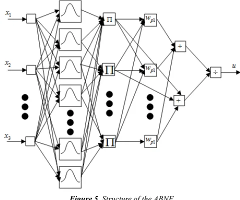
(34)

The structure for the AFNN is depicted in Fig. 5. It comprises of four layers:

Layer I: This layer is the input layer, i.e., introduces the inputs (x1, x2, ...,xm). This layer accepts the input values and transmits it to the next layer.

Layer II: In this layer the fuzzification process is performed and neurons represent fuzzy sets used in the antecedents’ part of the linguistic fuzzy rules. The outputs of this layer are the values of the membership functions, i.e.,ηij.

The membership of ith input variable to jth fuzzy set is defined by;

2

1 2

i ij

x m

v ij

e

η

−   − _ _  

=

(35)

Figure 5. Structure of the ABNF

Layer III: This layer is the fuzzy inference layer. In this layer each node represents a fuzzy rule. In order to compute the firing strength of each rule, and min operation is used to estimate the output value of the layer. i.e.,

( ) ( )

ij i ij i

i

x x

µ

=

∏

η

₍₃₆₎

where Π _{is the meet operation,} η_ij( )x_i are the degrees of the

membership function of the layer II and µ_ij( )x_i are the input values for the next layer.

Layer IV: This layer is the output layer. In this layer, the defuzzification process is made to calculate the output of the entire network, i.e., It computes the overall output of system.

4.1. Parameters Update rules

The fuzzy neural network learning is to minimize a given function or input and output values by adjusting network parameters. The gradient descent method is used to adjust the values of weights and the mean and variance of membership function. To minimize the error between the actual output value of the system and the desired value. For this purpose, gradient descent method is can be expressed as:

2 1

( - )

2 ref out

J= P P (37)

Where P_ref the desired output power of the system andP_out

is the actual output power of system. The updated amount for the wpiandηij can be obtained as:

( 1) ( )

-pi pi

pi

J

w t w t

w

γ ∂

+ =

∂ (38)

and

( 1) ( )

-ij ij

ij

J

m t m t

m

γ ∂

+ =

( 1) ( )

-ij ij

ij

J

v t v t

v

γ ∂

+ =

∂ (40)

Where γ is the learning rate.

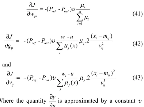
By taking the derivative of the above equations, it gives

1

-( - ) i

ref out m

pi

i i

J

P P

w

µ υ

µ = ∂ =

∂

_∑

(41)

2

- ( - ) .2( )

( )

i ij

i

ref out j

ij j

j

ij

w u x m

J

P P

g υ µ x µ v

∂ = −

∂

∑

(42)

and

2

3

- ( ) . ( )

( ) 2

- i

ref o

i ij

ut j

ij j

j

ij

w u J

P

x x

v P v

m

υ µ

µ

− ∂ =

∂

∑

(43)

Where the quantity y

u

∂

∂ is approximated by a constant υ

[34]. Equation (41)-(43) ate the required update equations of the AFNN.

5. Simulation Results and Discussion

The proposed adaptive AFNN control mechanism is applied on the 50 kW SOFC power plant system that has been modeled in MATLAB/Simulink. In order to check the performance and validation of the proposed controller, a short-duration active power transient study has been conducted considering SOFC stack under constant fuel flow. To estimate response of SOFC power system as grid real power demand change, step increase and decrease transients were applied on the system. The SOFC stacks have slow response to rapid and sustained load transients, observed throughout simulation. When a step change of power was experienced by utility grid, the power electronic inverter circuitry sensed these perturbations and the robust VSI control signal was effectively conditioned to able the SOFC plant to ramp up its output to meet required load demand. The results are compared with conventional PI controller to show the faster response time of proposed control strategy.

The SOFC based DG system is tested with step changes in the grid real power demand. These abrupt variations in the active power are for estimating the dynamic response of the SOFC system. A load model that represents subsequent changes in the active power demand is used to examine the response of the proposed model. The closed-loop strategy for SOFC is depicted in Fig. 6.

Figure 6. Closed-loop structure of AFNN based grid connected SOFC

In the Fig. 7, the active power reference is varied from

0.3p.u load to 1 p.u. at 0.1 sec and the response of the proposed AFNN model. It can be observed that reference active power demand curve is readily tracked by SOFC power output. This shows that proposed strategy is insensitive or robust against varying load conditions.

Figure 7. Active Power Tracking

A comparison of AFNN and PI controller is made to show the better performance of proposed control strategy. AFNN controller shows a rapid response, when it comes to tracking the active power demand. It can be observed that for a step change in active power from 0.3 p.u up to 1 p.u, the AFNN based SOFC takes almost 0.15 sec to acquire a new steady state condition. At the start, it is indicated that AFNN based SOFC take a bit timeto settle down to suitable values of system. Above system response show that AFNN control is capable of attaining rapid transient response with efficient rejection to load changes and achieve more stable response. It is observed that AFNN based grid-connected SOFC performs better than conventional PI controller. This shows that AFNN is computational strong and has ability to meet the desired response.

Figure 8. Load side voltage

Figure 9. Load side current

Figs. 10 and 11 show corresponding output response of the stack voltage and current of SOFC system when connected to grid. It is also observed that the stack voltage and stack current of SOFC changes accordingly during the variation in the load side power demands.

Figure 10. Stack voltage

Figure 11. Stack current

Figure 12. Hydrogen partial pressure

Figure 13. Water flow

Figure 14. Oxygen partial pressure

Figs. 15-17 depict the variations in the parameters of AFNN during online learning. This shows how the AFNN is flexible, computationally strong and his capability to meet desired demand of the grid.

Figure 15. Update parameters of mean of membership functions

Figure 16. Update parameters of variance of membership functions

Figure 17. Update parameters of weights

6. Conclusion

In this paper, an integrated model of SOFC system, connected to the electric power grid is presented. The detailed modeling of grid connected SOFC is described including inverter, filter, transformer and grid integration of SOFC is explained. Also, dynamical equation of partial pressure, stack voltage, stack current and temperature are explained. The main objected was to control and meet the active power demand variations occurring at load side. For this purpose, an AFNN is applied to the system. These changing demands schedules are sensed by SOFC system connected the infinite bus, and controller generate the required gate pulses for IGBTs of VSI for proper switching to meet the load demand. The performance of SOFC based DG system in grid connected mode with AFNN and PI controller have been compared and analyzed. The faster transient response and robustness of the proposed strategy is illustrated. Adaptive parameters update for efficient learning of the controller is also presented in the results.

References

[1] Y.T. Qi, B. Huang, K.T. Chuang, “Dynamic modeling of solid oxide fuel cell: the effect of diffusion and inherent impedance,” J. Power Sources, vol. 15, pp. 32-47, 2005.

[2] J. Larminie and A. Dicks, “Fuel Cell Systems Explained,”, 2nd ed. West Sussex, U.K: Wiley, 2003.

[4] N. Akkinapragada and B. H. Chowdhury, “SOFC-based fuel cells for load following stationary applications,” in Power Symp, 38thNorth Amer., Carbondale, IL, 2006,pp. 553–560. [5] Y. Zhu and K. Tomsovic, “Development of models for

analyzing the load following performance of microturbines and fuel cells,” Electr. Power Syst. Res., vol. 62, pp. 1–11, 2002.

[6] R. Kandepu, L. Imsland, B. A. Foss, C. Stiller, B. Thorud, and O. Bolland, “Modeling and control of a SOFC-GT-based autonomous power system,” Energy, vol. 32, pp. 406–417, 2007.

[7] F. Mueller, F. Jabbari, R. Gaynor, and J. Brouwer, “Novel solid oxide fuel cell system controller for rapid load following,” J. Power Sources, vol. 172, pp. 308–323, 2007. [8] J. T. Pukrushpan, A. G. Stefanopoulou, and H. Peng, Control

of Fuel Cell Power Systems: Principles, Modeling, Analysis and Feedback Design. New York: Springer-Verlag, 2004. [9] X.Wang, B. Huang, and T. Chen, “Data-driven predictive

control for solid oxide fuel cells,” J. Process Control, vol. 17, pp. 103–114, 2007.

[10] J. Padulles, G. W. Ault, and J. R. McDonald, “An integrated SOFC plant dynamic model for power systems simulation,” J. Power Sources, vol. 86, pp. 495–500, 2000.

[11] A. M. Murshed, B. Huang, and K. Nandakumar, “Control relevant modeling of planer s olid oxide fuel cell system,” J. Power Sources, vol. 163, no. 2, pp. 830–845, 2007.

[12] R. Lasseter, Dynamic Models for Micro-turbines and Fuel Cells, IEEE-PES Summer meeting," vol.2, pp. 761-766, July 2001.

[13] K. Ro, and S. Rahman, Two-Loop Controller for Maximizing Performance of a Grid-Connected Photovoltaic-Fuel cell Hybrid Power Plant, IEEE Trans. Energy Conversion, vol. 13, Issue 3, pp. 276-281, September 1998.

[14] Don B. Nelson, M. Hashem Nehrir, and Victor Gerez, Economic Evaluation of Grid Connected Fuel-Cell Systems IEEE Transactions on Energy Conversion,"vol. 20, no. 2, June 2005.

[15] W. Du, H.F.Wang, Effect of grid-connected solid oxide fuel cell power generation on power systems small-signal stability," IET Renewable Power Generation, 31st January 2009.

[16] F. Jurado, “Predictive control of solid oxide fuel cells using fuzzy Hammerstein models,” J. Power Sources, vol. 158, pp. 245–253, 2006.

[17] Sanandaji, B. M., Vincent, T. L., Colclasure, A. M., &Kee, R. J., “Modeling and control of tubular solid-oxide fuel cell systems: II. Nonlinear model reduction and model predictive control,” Journal of Power Sources, vol. 196, no. 11, pp. 208-217, 2011.

[18] M. Singh and A. Chandra, “Real-time implementation of ANFIS control for renewable interfacing inverter in 3P4W distribution network,” IEEE Trans. Ind. Electron., vol. 60, no. 1, pp. 121–128, Jan. 2013.

[19] García, P., Garcia, C. A., Fernández, L. M., Llorens, F., &Jurado, F.,“ANFIS-Based Control of a Grid-Connected Hybrid System Integrating Renewable Energies, Hydrogen

and Batteries,” IEEE Trans. Industrial Informatics, vol. 10 no. 2, pp. 1107-1117, 2014.

[20] T. A. Johansen, R. Shorten, and R. Murray-Smith, “On the interpretation and identification of dynamic Takagi–Sugeno fuzzy models,” IEEE Trans. Fuzzy Syst., vol. 8, no. 3, pp. 297–313, Jun. 2000.

[21] T. A. Johansen and R. Babuska, “Multi objective identification of Takagi– Sugeno fuzzy models,” IEEE Trans. Fuzzy Syst., vol. 11, no. 6, pp. 847– 860, Dec. 2003.

[22] G. Feng, “A survey on analysis and design of model-based fuzzy control systems,” IEEE Trans. Fuzzy Syst., vol. 14, no. 5, pp. 676–697, Oct. 2006.

[23] T. J. Zhang, G. Feng, and J. H. Lu, “Fuzzy constrained min-max model predictive control using piecewise Lyapunov functions,” IEEE Trans.Fuzzy Syst., vol. 15, no. 4, pp. 686– 698, Aug. 2007.

[24] T. J. Zhang, G. Feng, J. H. Lu, and W. G. Xiang, “Robust constrained fuzzy affine model predictive control with application to a fluidized bed combustion plant,” IEEE Trans. Control Syst. Technol., vol. 16, no. 5, pp. 1047–1056, Sep. 2008.

[25] T. J. Zhang, G. Feng, and X.-J.Zeng, “Output tracking of constrained nonlinear processes with offset-free input-to-state stable fuzzy predictive control,” Automatica, vol. 45, no. 4, Apr. 2009.

[26] J. L. Bernal-Agustín and R. Dufo-López, “Simulation and optimization of stand-alone hybrid renewable energy systems,” Renew. Sust. Energ.Rev., vol. 13, no. 8, pp. 2111–2118, Oct. 2009.

[27] M. A. Akcayol, “Application of adaptive neuro-fuzzy controller for SRM,” Adv. Eng. Softw., vol. 35, no. 3-4, pp. 129-137, Mar. 2004.

[28] Handbook. Fuel Cell, (2004).EG & G Technical services. Inc., USDOE, 7-18.

[29] Wu, X. J., Zhu, X. J., Cao, G. Y., &Tu, H. Y, Dynamic modeling of SOFC based on a T–S fuzzy model. Simulation Modeling Practice and Theory, vol. 16, no. 5, pp. 494-504, 2008.

[30] Zadeh, L. A, Fuzzy sets. Information and control, vol. 8, no. 3, pp. 338-353, 1965.

[31] Takagi, T., &Sugeno, M. (1983, July). Derivation of fuzzy control rules from human operator’s control actions. In Proceedings of the IFAC symposium on fuzzy information, knowledge representation and decision analysis (vol. 6, pp. 55-60).

[32] Ying, H, Fuzzy control and modeling: analytical foundations and applications. Wiley-IEEE Press, 2000.

[33] Sayed T., Tavakolie A. and Razavi A.,“Comparison of adaptive network based fuzzy inference systems and B-splineneuro-fuzzy mode choice models,” Journal of computing in civil engineering, vol. 17, no. 2, pp. 123–130, 2003.