LTR – MDTS structure – A structure for Multiple
Dependent Time Series Prediction
Predrag Pecev1and Miloš Rackovi´c2
1 Unversity of Novi Sad, Technical faculty "Mihajlo Pupin"
Ðure Ðakovi´ca BB, 23000, Zrenjanin [email protected]
2
Unversity of Novi Sad, Faculty of Sciences Trg D. Obradovi´ca 3, 21000, Novi Sad
Abstract. The subject of research presented in this paper is to model a neural net-work structure and appropriate training algorithm that is most suited for multiple dependent time series prediction / deduction. The basic idea is to take advantage of neural networks in solving the problem of prediction of synchronized basketball referees’ movement during a basketball action. Presentation of time series stem-ming from the aforementioned problem, by using traditional Multilayered Percep-tron neural networks (MLP), leads to a sort of paradox of backward time lapse effect that certain input and hidden layers nodes have on output nodes that correspond to previous moments in time. This paper describes conducted research and analysis of different methods of overcoming the presented problem. Presented paper is essen-tially split into two parts. First part gives insight on efforts that are put into training set configuration on standard Multi Layered Perceptron back propagation neural networks, in order to decrease backwards time lapse effects that certain input and hidden layers nodes have on output nodes. Second part of paper focuses on the re-sults that a new neural network structure called LTR - MDTS provides. Foundation of LTR - MDTS design relies on a foundation on standard MLP neural networks with certain, left-to-right synapse removal to eliminate aforementioned backwards time lapse effect on the output nodes.
Keywords:MLP, Multiple Dependent Time Series, LTR - MDTS structure, Train-ing parameter influence, Neural Network Configuration, TrainTrain-ing Set Configuration and Optimization.
1.
Introduction
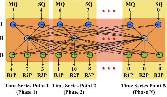
a complete input pattern. In this way, the input layer of the neural network represents a complete time series, and time is propagated along the neural networks layers, for exam-ple, from left to right as shown in Fig. 2 in Chapter 3. At the output of the neural network a vector is expected that represents the movement of three basketball referees in a form of three dependent time series. Following this approach output nodes of neural networks also form appropriate key points in the form of a time series for movement of basketball referees. From previously said it can be concluded that through the entire neural network time flows along layers through the neural network nodes from left to right.
The above is quite a change from most currently available approaches, where, for a range of input values that represent time series, using a variety of techniques and the transformations of input data, only one output value is reasoned as a next moment in time series. In this paper we propose an approach where for one complete input time series, three complete dependent (parallel) time series are being reasoned. Aforementioned three complete defendant output time series are occurring in the same time interval as an input one, and not only that they are codependent among themselves, they are also codependent on the input time series. Also, in when we analyze most currently available approaches regarding time series, it can be concluded that values of parameters that represent the input time series of a neural network are in the same domain as the output ones. This is not the case in our approach since input values of a neural network present movement of a ball on a basketball court, while the output is movement of referees along touchline of a basketball court.
At first glance, it seems that the feed forward neural network in which it is natural that the information is run through layers, from input to output layer, not taking into account which nodes are located on the left and right side of a neural network, is utterly unsuitable for solving of a presented problem. When a solution for a presented problem is being calculated, due to proposed time flow that goes along layers through neural network, propagation of information backward in time is allowed, which seems unacceptable and contradictory to the actual situation. This means that previous moment in time is affected by next moments in time which could be considered to be somewhat of a paradox. But if we consider the real problem, which is the movement of basketball referees in a way that allows them to, as best as possible, examine the position of the ball and the general situation on the basketball court, we noticed that very often in basketball some of the widely known standard plays are run. Those plays are very well known by referees, and very often they do not respond exclusively to the current position of the ball on the court, but rather move on the basis of their prior knowledge or at least expectations of where the ball will be in the next few moments.
mo-ment in time. Based on what was previously said, it is clear that we want to reduce effects of later moments in time to the previous and current moments in time since traditional MLP structure allows this feature. In this paper we also propose LTR – MDTS (Left to Right Multiple Dependent Time Series) structure of the neural network that is more suit-able for solving a presented problem. The idea is to solve a presented problem through usage of aforementioned classes of neural networks and to later compare the results.
Previous exposure leads to another direction in the entire study, which refers to the verification of the implemented prediction model and trained neural networks in general. Although the training algorithm that is used in the prediction of referees’ movement for the desired correct position of a referee in certain key points used a fixed position along the touchline of a basketball court, it is clear that the real problem is not the positioning of referees in the desired fixed points, but placement of basketball referees so they can at any time oversee the play as best as they can, considering all key aspects of the play. On the one hand, we are not sure whether the referee will oversee the play the best way possible, even if he is the desired position, as different positions of the players during the play, which were ignored in the process of training the neural network, can lead to obstruction of visual field of basketball referees. On the other hand, sometimes the referees will be able to oversee the play very well, even they are not placed the desired position, but placed in the position that is one or two meters further from a desired position.
Based on what was previously said it can be concluded that the existing methods of validating the performance of neural networks in this case are not adequate, and that, therefore, a special criterion that will assess neural network performance based on pre-sented problem domain must be created. The above criterion is called SRC criterion (Sat-isfactory Results Criteria). SRC criterion implemented two important aspects:
• Synchronized movement of basketball referees, which is not allowed to considerably deviates from its ideal trajectory compared to other referees along the touchline of a basketball court
• Permitted deviation from the ideal desired position of basketball referees in a partic-ular spatial range
However, the main validation criterion represents a simulation of the horizontal field of view of basketball referee through which, based on all the elements of basketball action it is determined, whether, basketball referees, based on the reasoned synchronous move-ment could adequately oversee the basketball action. Aforemove-mentioned validation will not be presented in this paper since they constitute the final phase of neural network validation which is run when presented neural network shows satisfactory results when evaluated with SRC criterion. This paper presents the behavior of the traditional MLP and proposed LTR - MDTS structures in the domain of the present problem that are validated through the SRC criterion.
2.
Related work
al. [7], Zhang et al. [8], Giles et al. [9], Lai et al. [10], Khashei et al [11] and Patra et al. [14].
Works of Teo et al [12] and Romdhane Ons et al. [13] show that multilayered percep-tron can be used for Time Series prediction. Teo et al. [12] emphasize the value of Weight Initialization, and show that weight initialization influences successfulness of training neural networks, while Romdhane Ons et al. [13] present an algorithm for automatic de-sign of optimal neural network models for time series prediction, that is based on back propagation and genetic algorithms. In a way, our work is similar to works of Romd-hane et al. [13] since the foundation of our research, regarding neural networks relies on forming an algorithm, methods and neural network structure in order to produce one or multiple related time series, based on an input of one time series, that happens in a very short time period (24 seconds) and can be considered somewhat chaotic as described in work of Teo et al. [12] regarding Mackey-Glass Chaotic Time Series.
Wan et al. in paper [2] present solutions that are similar to a solution presented in this paper and provide a common framework to derive popular algorithms, including back propagation and back propagation through time, without a single chain rule expansion. They also provide simple intuitive relationships between such algorithms as real time recurrent learning, dynamic back propagation and back propagation through time.
Vintan et al. in paper [3] use MLP (Multilayered Perceptron) back propagation neural networks to predict a person’s movement within a building based on a Time Series. Najim et al. in their work [18] present a multilayered perceptron back propagation approach to forecast electric power load curves based on various parameters, and presents a neural network for short-term load forecasting while Abuadlla et al. in their work [19] deal with issues of attacks on large network and computer systems where MLP network was used to select time windows where attacks are more probable based on the significant changes in traffic over time.
Ivankovi´c et al. [1], determined that the most common elements of a basketball game are shoots for 2 points under the hoop and defense rebound, through the analysis of the first B basketball league for men from 2005 and 2010, using feed forward neural network. Similar research is presented in paper by Ratgeber et al. [16] regarding First senior leagues for men and for women in Serbia during the 2011/2012 season where it is stated that in both leagues, defensive rebounds have the strongest influence on winning the game. Also Ivankovi´c et al. [17] present a solution for automatic player position detection in basketball games, through position estimation and usage of Latent SVM, where, based on the recordings of basketball games positions of basketball players can be determined, and possibly converted into basketball scenarios for a certain basketball action that can be used for automated training and test set creation.
Loeffelholz et al. [20] in their paper describe how through the usage of various neu-ral networks, such as feed forward, radial, probabilistic, regressive neuneu-ral networks, and also through the fusion of mentioned types of neural networks, an outcome of a game can be predicted, emphasizing that the predictions of the trained neural networks were more precise compared to the basketball expert’s predictions. In conclusion, trained neural net-works predicted the outcome of the game correctly in 74.33 % cases, while the basketball experts were precise in 68.7% cases.
mainstream solutions input time series, through deployment of input wavelet transforms, genetic algorithms, backward time series flow, etc., usually produce one output time se-ries, or a next point in time, which is opposite to our case where it produces 3 complete different but dependent time series.
3.
Traditional MLP Approach
Foundations of the developed solution regarding proposed basketball court partitioning, MLP neural network structure, neural network evaluation criteria, training methods and training and test sets structure, were previously published in paper by Markoski et al. [15] and will be referred here in order to get a better understanding of the terminology, methods and results that are presented in this paper. Also we would like to emphasize that appropriate original training and test sets were obtained by first author of Markoski et al. [15], a basketball delegate for First Female Serbian Basketball League in collaboration with a team of basketball referees and coaches that he selected.
From scenarios of basketball actions, pairs of input and output vectors for the neural network were generated, thus forming training and test sets. Dataset for neural network training consists of 43 basketball actions that are taught on basketball training sessions with appropriate movement of basketball referees during those basketball actions. Since aforementioned basketball actions from training set are played on basketball training ses-sions it is clear that they hold expert knowledge provided by aforementioned basketball experts. At this point, it is clear that training set, regarding number of patterns is consid-ered to be quite small, and can produce the effect of overfitting, yet since it holds expert knowledge we have proceeded with our research. The test set consists of the 20 actual situations from the official basketball games that are actually played. Movement of bas-ketball referees in the training, as well as in the set for testing the neural network were established taking into account the movement of players on the basketball court during the basketball action.
To ensure that training and test sets were appropriate, each basketball action was first run through a simulation of a human field of vision, which is not presented in this paper. If position of basketball referees in any point in time produced unsatisfactory results from the aspect of successful overseeing a basketball action, paths of basketball referees for that action were slightly modified, by moving a referee a bit, up or down the assigned court lines.
Fig. 1.Basketball court partitioning
The court position of the ball is described through arranged pair [main quadrant, sub quadrant]. The main quadrant parameter will pinpoint to one of 6 prime quadrants that are defined by FIBA as presented in paper Markoski et al. [15]. In Fig. 1, main quadrants are marked with capital 1 through 6 numbers. Sub quadrant parameter pinpoints to one of 4 subsections of the quadrant which are not defined by FIBA. They are implemented for precision positioning and are marked with the lower case 1 through 4 numbers. Since placement of sub quadrants within a main quadrant in paper Markoski et al. [15] proved to be not so functional for the end user, modified sub quadrant placement that has been used in paper Pecev et al. [21] has been used here as well. In that manner, we can state that one key point is described with arranged pair [main quadrant, sub quadrant] which indicates the positions of the ball and the 3 man referee system [referee1pos, referee2pos, referee3pos], where for example, referee1pos identifies referee number 1 in a fixed posi-tion on 12 point scale, etc.
Since maximum length of the input vector of neural network is 30 elements, or 15 key points, noted as t1, t2 . . . tn, where max(n) = 15, defined by an ordered pair [main quadrant, sub quadrant], all values of input vector are first set to 0, and then they are filled, starting from the left-hand side, by ordered pairs, taking care to follow structure of a basketball action [quadrant-t1, subquadrant-t1, quadrant-t2, subquadrant-t2. . . ] etc. The output vector is formed in a similar way. Since maximum length of the output vector of the neural network is 45 elements, or 15 key points, noted as t1, t2 ... tn, where max(n) = 15, defined by ordered three [referee1pos, referee2pos, referee3pos], all values of the input vector are first set to 0 and then they are filled, starting from the left-hand side, by ordered threes, taking care to follow structure of a basketball action [referee1pos-t1, referee2pos-t1, referee3pos-t1, referee1pos-t2, referee2pos-t2, referee3pos-t3,. . . ] etc.
Fig. 2.Structure of AForge .NET MLP neural network
the basketball court. Both input and output vectors follow the previously stated rules that define the order of elements such as main quadrant and sub quadrant numbers in and input vector of a neural network, as well as referee positions in the output vector of a neural network. Aforementioned is shown in Fig. 2.
These MLP Back Propagation neural networks are implemented with AForge.NET neural network framework. Each layer trained and tested neural network was activated by
Bipolar Sigmoid function with 0.5 Alpha offset value, here stated asf(x) = 2
1 +e−α×x- 1 , learning rate was declared as 0.25 while momentum was considered relatively high and was set to 0.7. At first traditional method of defining number of iteration was used, and later, after we concluded that due to random initiation of neuron weights we should try to search and test for configurations that will not succumb to the effects of local minima, and if they do succumb to local minima, they succumb with the highest possible marks on the Satisfactory Results Criteria that will be explained later in this paper.
In order to generate a certain number of neural networks and find the best configura-tion of a neural network that will produce optimal movement paths for basketball referees, a large number of neural network configurations (1048575) were generated. Generated neural networks configurations had from 1 to 20 hidden layers, and in each one of these possible 20 layers there could be from 1 to 20 neurons per each layer. Each neural net-work, regardless of its configuration, will be given 10 minutes for the training process, thus enabling a neural network to potentially succumb to the local minima even with such high momentum. During the training process, various parameters were followed, such as the time it takes for the percentage of training a neural network to exceed 50 or 80 percent tested with a Satisfactory Results Criteria. Satisfactory Results Criteria or SRC in short is a specially devised criterion that we use to rate the performance of trained neural net-works. SRC criteria is applicable only within a domain of a presented problem and will be reviewed later in this paper.
and by structure of perceptron neural networks impossible, to avoid influence of other neuron weights while forming an output. Thus, a method of training a neural network was formed based on the way a training set is organized and run through a neural network in order to decrease the influence of neurons that, regarding time series problem in general, should not influence on reasoning and calculation of the sequential output time series. E.g. weights of the neurons that mostly calculate positions of referees in key point 5 should not influence neurons that mostly calculate positions of referees in key point 3, although, neurons that mostly calculate positions of referees in key point 3 should influence neurons that mostly calculate positions of referees in key point 5. We call this rule Left-To-Right Weight Propagation. This rule is a foundation for a neural network structural organization model we called LTR - MDTS model which will also be presented later in this paper.
3.1. Training Methods, Training set configuration and optimization
Presented training methods are:
• Traditional back propagation algorithm
• Sequential repetition with progressive action development
In order to speed up the training process, values for quadrant, sub quadrants and ref-eree positions are divided by a maximum value from their range of values or domain. It was previously noted that values for the main quadrant entity range between 1 and 6, val-ues for sub quadrant range between 1 and 4 valval-ues for referee positions and range from between 1 and 12. This means that before the training process starts, input and output patterns are converted into values that range from 0 to 1, and trained to produce outputs in the noted range. During the testing phase, input parameters are first converted into values that range from 0 to 1, and then, output values, that also range from 0 to 1 are expanded, by multiplying each value by 12 and rounding it up to the nearest whole number, and then evaluated. We have chosen this approach and standard normalization scheme in order to work with values that are in rage from 0 to 1 since, as activation functions we use Alpha Sigmoid (Bipolar) function that produces values from a -1 to 1 interval, and we aim for values from a positive range of an aforementioned interval.
a sequence of patterns [t1], [t1,t2], [t1,t2,t3], [t1,t2,t3,t4], where tn is action key point and [t1, . . . tn] is a pattern. Advantages of neural network training using method of Sequential repetition with progressive action development, in comparison to classical method, are summarized in two points:
• Decreased influence of input node sequence values to values of output node sequence values that are in correspondence with previous moments in time. These solutions are closer to expected, common-sense logical solutions for particular situation than solutions given by the neural network trained by the classical method.
• Application of the Sequential repetition method with progressive action development over the same set of patterns for neural network training, quantitatively multiplied number of patterns used for its training. New patterns, formed during neural network training, were formed as subsets of existing patterns. These are not essentially new informations, yet they are helping to emphasize time flow of a basketball action.
Neural networks, trained by these methods, had in all cases correctly established cor-relation between number of input and output points as input and output vectors, which was a first indication that it is possible to decrease influence of unwanted nodes in order to produce satisfactory results. The neural networks understood that a length of a pattern is dependent on the sequence of zeroes that fills in the rest of the input and output vector, thus forming appropriate connections based on the values from the beginning of a vector, to the point where array of zeroes begin.
4.
SRC – Satisfactory results criteria
Since training and tests sets were created using an application for drawing basketball actions, patterns were formed by an approximation for both referee movement and ball position. Regarding movement of basketball referees, on a drawn basketball action, based on a position of a basketball referee, referee was moved to the nearest point on a fixed scale of referee movement. This way first approximation in a presented model was made. Next, from Fig. 1 it can easily be seen that a basketball court is divided into 24 areas of equal size that are organized (marked) in aforementioned manner. Keeping in mind that an ordered pair [quadrant, sub quadrant] approximates a large number of potential ball positions in a certain quadrant, and in a rather crude way separates itself from other quadrants thus providing a rather strict framework for modeling real life situations, it was decided that appropriate criteria for assessing outputs of neural networks was needed.
It was already mentioned in previous chapters that the primary goal problem solving is not just simple fixed positioning of the exact desirable referee position somewhere down the court line, but reaching an optimal position to closely monitor all the key aspects of a play action at all times. That is why, for the evaluation of neural network successfulness, a specific criteria is deployed which does not allow referee desirable position to deviate +/-2 notches from the optimal spot. Optimal spots are defined as approximated desired referee positions for basketball actions from training and test sets that are formed on the basis of provided expert knowledge.
Table 1.Input vector of neural network
Point t1 t2 t3 t4
Index 0 1 2 3 4 5 6 7 8 9 10 . . . 29 I.V. 1 4 6 2 4 3 5 1 0 0 0 . . . 0
Table 2.Output vector of the neural network that will be evaluated
Point t1 t2 t3 t4
Index 0 1 2 3 4 5 6 7 8 9 10 11 12 . . . 44 O.V.(R) 4 7 3 1 4 8 5 10 1 12 6 7 0 . . . 0
O.V.(E) 4 6 5 1 3 9 5 8 1 9 6 7 0 . . . 0
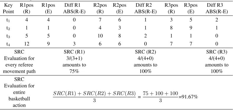
Table 3.Output vector of the neural network that will be evaluated Key Point R1pos (R) R1pos (E) Diff R1 ABS(R-E) R2pos (R) R2pos (E) Diff R2 ABS(R-E) R3pos (R) R3pos (E) Diff R3 ABS(R-E)
t1 4 4 0 7 6 1 3 5 2
t2 1 1 0 4 3 1 8 9 1
t3 5 5 0 10 8 2 1 1 0
t4 12 9 3 6 6 0 7 7 0
SRC Evaluation for every referee movement path SRC (R1) 3/(3+1) amounts to 75% SRC (R2) 4/(4+0) amounts to 100% SRC (R3) 4/(4+0) amounts to 100% SRC Evaluation for entire basketball action
SRC(R1) +SRC(R2) +SRC(R3)
3 =
75 + 100 + 100
3 =91.67%
neural network is assessed is shown in Table 3. Input vector is shown in Table 1 while expected output vector marked O.V. (E) and reasoned output vector marked O.V. (R) are shown in Table 2.
of basketball referees during an entire basketball action, each reasoned movement of a basketball referee must be reasoned with a SRC criteria, and only if a movement of all referees get a passing grade of 66.00%, an average grade will be calculated that presents a measurement that indicates if that particular movement could be considered satisfactory. If aforementioned grade for each reasoned output pattern passes 66.00%, that result is ac-cepted as satisfactory. Since training set has 43 basketball actions, when a certain neural network states that percentage of successful training is 95.34% it actually says that output patterns of 95.34% actions (41/43) from training set of a neural network are considered to be satisfactory. The very same is also applied on the neural network test set.
Depending on the allowed deviations we use two types of SRC validations:
• Weak SRC criteria – Allowed deviation is +/- 2 notches and, in this chapter used to explain basic structure of SRC criteria
• Strict SRC criteria – Allowed deviation is +/- 1 notches
Because one half of the basketball court is, regarding their touchlines, divided into 11 equal sections, possible referee distance between two points, due to basketball court dimensions, is between 1.27 and 1.36 meters which averages to cca 1.32 meters. That measurement satisfies the criteria of a real life problem described in the introduction. Later on, when comparative tests are presented, we will address the aforementioned methods with the goal of pointing out certain observations.
Also, if we try to evaluate the successfulness of neural networks by rating it with a zero deviation SRC criteria, where it is expected from a network to generate referees’ output positions in exact values without deviations, results that any neural network that is presented in paper Pecev et al. [21] or in this one would be considered utterly unusable since they rarely or never produce exact desired output. Previously stated is a feature of both MLP structures and, presented later in this paper, LTR – MDTS structures. However, since it was stated that our goal was not only to place basketball referees in optimal positions, or as closer to optimal positions, while emphasizing synchronized movement of basketball referees and real life situations, we have decided to use SRC criteria with deviations opposed to SRC criteria without deviation. Based on the previously said any other criteria that do not allow deviations such as MSE (Mean Squared Error) or RSS (Residual Sum of Squares) were not taken into account since their application does not fit well into a structure and basic goal of solving a presented problem while keeping an emphasis on previously mentioned features.
5.
LTR - MDTS Model
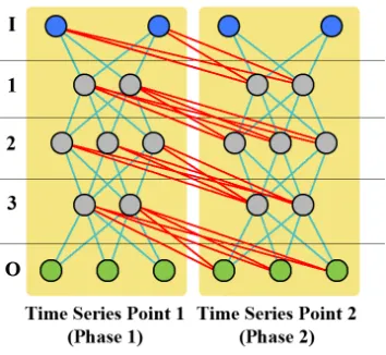
LTR – MDTS model stands for Left to Right – Multiple Dependent Time Series model. Structure of the presented model, shown in Fig. 3, resembles a model of multilayered perceptron neural network with certain key differences.
Fig. 3.Structure of LTR – MDTS model
between neurons that are dyed light blue do not deviate in any manner from traditional multilayered perceptron structure. Sole purpose of this model is to form a structure that, on the structural level of a neural network, replicates dependent time series structure. Pre-viously it was already stated that every point in time, or a state, depends on all of that point previous points. For example, if we have 3 states, aligned sequentially in a 1→2 →3 manner, output of point 3 depends on both inputs of point 1 and 2.
Here we have defined Left-To-Right Weight Propagation, and Left-To-Right Bonds. Dyed red, in Fig. 3, Left-To-Right bonds are presented. Those bonds transfer neuron out-put values from left to right, connecting all neurons of any layer within any segment of a neural network to all neurons in the next layer within segments that are located to the right from that particular segment of a neural network, thus enabling, from the structural aspect of neural network, dependent time series structure. Structures of hidden layers within seg-ments that represent Time Series Points can be identical, regarding numbers of neurons per layer, as shown in Fig. 3, or they can be different. The only bounding factor of pre-sented structure is that all segments of a neural network must have the same number of layers in order to form Left-To-Right bonds.
within a neural network trainer. Also, on the basis of Delta rule we are calculating new neuron weights and bias correction values.
Random neuron weight and bias initialization is done based on Marsaglia polar method that is used for generating pairs of pseudo random numbers. Random number generator that uses Marsagila polar method is formed based on the lectures given by prof. Mike Giles [22]. During implementation only first generated number is used, while the sec-ond one (spare) is disregarded. Also, during calculation of a random number based on Marsagila polar method mean value of 0.0 and standard deviation of 1.0 was used. By examining values of aforementioned parameters it is clear that generated values produced by Marsagila polar method, and used for neuron weight and bias initialization, were not affected by mean or standard deviation values.
Modification of Back Propagation algorithm is called NNTL Back Propagation algo-rithm where NNTL stands for No Node Time Lapse and emphasizes forming of values for changing neuron weights and biases as it is described in Karmilasari, S. M. [23] with sim-ple check to see if neurons from current and previous layer are connected. In the context of the problem that is being solved, aforementioned acronym NNTL was added in order to easily differentiate results, yet since it presents a modification of a traditional Back Prop-agation algorithm in order to emphasize existence of missing neural network synapses, we believe that addition of aforementioned acronym is justified. Missing synapses bond effect is obtained by forming two matrixes that consist only logical values and indicate weightier a certain neuron from one layer is connected to a neuron from a previous layer (if a signal is run forward – Feed Forward) or next layer (if a signal is run backward – Feed Backward). Based on what was previously said it can be concluded that LTR – MDTS structure is, in its core, structure of a multilayered perceptron, or a simple MLP neural network that is extended with previously described matrixes in order to define sig-nal propagation through a neural network.
NTL Back Propagation algorithm, where NTL stands for Node Time Lapse, points to an alternative modification of a Back Propagation algorithm that besides mechanism for simulating effects of missing synapses implements backward error propagation on the basis of individual calculations for each signal as it reaches desired neuron. During aforementioned calculation it is very important that, for each signal that reached desired neuron from previous layer (and neuron error), a sum of weight and first derivative of a neuron activation function is made. Let’s assume that the output of one neuron in back-ward error propagation phase is influenced by 4 neurons from previous layer. Markings, indexes and term meaning of current and previous have remained the same as described in the presentation of NNTL Back Propagation algorithm. First, in a left to right order, error of a first neuron is taken into consideration, evaluated with a first derivative of a neu-ron activation function, and that value is saved. Next, on a saved value, error of e second neuron is added, and again, evaluated with first derivative of a neuron activation function, and saved yet again. Aforementioned is repeated until all signals and neuron weights from all connected neurons from previous layer have reached its destination to the neuron in the current layer. When the last signal of connected neurons has reached its destination, neuron error value for that particular neuron is formed.
training, since, in presented case, depending on how many connections neuron has, and to which key point neuron belongs, influence of that particular neuron is either heightened or lowered in correspondence to appropriate key point (phase). It is obvious that in that way, the largest influence present neurons that are located on the left side of a neural network, or neurons that are calculating starting points of basketball referee paths, while influence of neurons will slowly decline towards the ending of a basketball action (time series).
In order to achieve greater similarity between LTR – MDTS and MLP neural network structures, each neuron from the same layer has the same activation function. Also each layer of a LTR – MDTS neural network also has the same activation function, as is the case with MLP neural networks. In case of LTR – MDTS neural network, a Fast Sigmoid activation function is selected since it produces best results, its computational costs are low and it computes faster than Bipolar Sigmoid function that was used in MLP neural
networks. Fast Sigmoid function is stated as:f(x) = x
|x|+ 1 while its first derivative is
stated as:f’(x) = 1
(|x|+ 1)2 . Also, activation functions such as Algebraic Sigmoid, TanH and Gaussian have been taken into consideration but disregarded since they provided re-sults that were not as satisfactory as rere-sults obtained using Fast Sigmoid. In paper Menon et al. [24] TanH and Algebraic sigmoid functions are described, characteristics of Fast Sigmoid function are described in paper Beiu et al [25], while foundations of Gaussian function are well known and will not be explained or referenced in this paper.
6.
Results
In this chapter, the two subsections will present the results of the presented solutions and models through their evaluation. The first subsection presents a comparison of the results that traditional MLP neural networks, trained by aforementioned algorithms, produced based on the SRC criteria. The second chapter presents an evaluation of LTR - MDTS neural networks that are trained based on the previously established MLP settings that we consider to be good, and highlights the nature of LTR - MDTS structure in terms of parameter values that are needed in order to LTR - MDTS networks provide the best performance.
Depending on the method of training the neural network, the best neural network will be selected on the basis of performance they achieve on both training and test sets. Fol-lowing tables have clearly distinguished four groups of columns based on the deviation within SRC criteria. When we want to point out to neural networks that produced best results from already selected best neural networks based on number of hidden layers we emphasize: neural network configuration name (which consists of ann prefix meaning Ar-tificial Neural Network and ordinal number of configuration out of previously mentioned 1048575 neural networks), number of hidden layers and marks presented in columns Trained and Tested.
6.1. Validation of MLP Neural Networks and proposed algorithms
networks that are mentioned in paper Pecev et al. [21] and have up to 20 hidden layers. Each of selected 12 neural networks represents a class of neural networks that differ on the number of hidden layers ranging from 1 to 12 hidden layers. Reasons for disregarding neural networks that have more than 12 hidden layers are presented in paper Pecev et al. [21] and thus will not be presented in this paper. However, training and test sets that were used for training of neural networks that are presented in this paper were slightly modified in comparison to original training and test sets that were used for training of neural net-works that are described in paper Pecev et al. [21] and for initial results and concepts that are presented in Markoski et al. [15]. Modified training and test sets and random neuron weights initialization have shown its influence on the performance of retrained selected neural networks using same settings as previously described. Also different neural net-work model was used. In paper Pecev et al. [21] neural netnet-works supported basketball actions that had up to 15 key points or phases thus forming input vectors that have 30 elements and output vectors that had 45 elements. Presented neural networks in this paper are based on a modified neural network model that supports up to 12 key points, since both original and modified training and test sets consist of basketball actions that have from 3 up to 12 key points. Based on what was previously said it can be concluded that neural networks presented in this paper work with input vectors that have 24 elements while output vectors have 36 elements. However, even with aforementioned alterations, after thorough analysis, almost identical conclusions, which will be presented later in this chapter, were deducted.
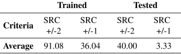
Table 4. Average marks that AForge.NET MLP neural networks that are trained with traditional Back Propagation Algorithm scored on both weak and SRC criteria
Trained Tested
Criteria SRC
+/-2
SRC +/-1
SRC +/-2
SRC +/-1
Average 91.08 36.04 40.00 3.33
When we consider weaker SRC criterion, and neural networks that were trained with traditional Back Propagation algorithm, based on the data from Table 4, the best results are obtained with neural network ann1560 which has 5 hidden layers with values of 97.67% on training and 50.00% on the test set. When we consider a strict SRC criterion, and the aforementioned class of neural networks, although neural network ann15472 with 8 hidden layers does not produce best results regarding training set, the very same has been chosen as a representative of neural networks that provide best results regarding test set in comparison towards results that were obtained on a training set. Aforementioned neural network ann15472 with 8 hidden layers provides values of 27.90% on training set and 10.00% test set.
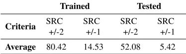
Table 5. Average marks that AForge.NET MLP neural networks that are trained with Method of Sequential Repetition with progressive action development scored on both weak and strict SRC criteria
Trained Tested
Criteria SRC
+/-2
SRC +/-1
SRC +/-2
SRC +/-1
Average 80.42 14.53 52.08 5.42
on training and 65.00% on the test set. On the basis of a strict SRC criterion, best results provides neural network ann51458 network with six hidden layers and values of 13.95% for training and 10.00% on the test set.
By comparing results from Tables 4 and 5 it can be concluded that Method of Se-quential Repetition with Progressive Action Development provides far better results com-pared to traditional Back Propagation algorithm when rated with both weaker and stricter SRC criteria regarding test set as described in paper Pecev et al. [21]. Here it has been noted that neural networks that were trained using traditional Back Propagation algorithm showed better results on training set than neural networks that were trained using Method of Sequential Repetition with Progressive Action Development regarding both weak and strict SRC criteria. Compared to results that were published in paper Pecev et al. [21] there is a slight difference in general behavior of presented algorithms regarding training set and marks that were obtained based on the weak SRC criteria where Method of Se-quential Repetition with Progressive Action Development provided slightly better results compared to traditional Back Propagation algorithm.
However, in both presented cases it was noted that training neural networks with Method of Sequential Repetition with Progressive Action Development provided better results regarding test set in general, which was one of the desired goals of a devised al-gorithm. Regarding results presented in Pecev et al. [21], there are neural networks that were trained using traditional Back Propagation algorithm and produce results that could be considered somewhat satisfactory, so, it can be said that aforementioned algorithm can also be, to some extent, used for solving the presented problem. However, based on pre-sented facts in paper Pecev et al. [21] clear emphasis is on the usage of a counterpart algorithm for training neural networks with MLP structure which is in this paper also confirmed.
Values of parameters that produced satisfactory results, in this paper stated in sec-tion 3, and noted as MLP Good Settings and considered to be adequate for training of AForge.NET MLP structures in the domain of a presented problem. Several tests have been conducted in order to form aforementioned statement, and foundations of those tests are described within the next chapters.
6.2. Validation of LTR – MDTS Neural Networks and proposed algorithms
The aforementioned configurations of neural networks are trained with NNTL Back Prop-agation algorithm and NTL Back PropProp-agation algorithm. We did not train LTR – MDTS neural networks with Method of Sequential Repetition with Progressive Action Develop-ment since LTR – MDTS neural network provides physical structure for effects that were simulated with aforementioned training algorithm on MLP neural networks.
For each test presented in this chapter all 128 configurations of neural networks were trained and classified by number of hidden layers. From each class of neural networks, regarding number of hidden layers, one neural network that we consider that shows best performance was selected. The same method was initially applied when working with MLP networks so we believe that applying the same principle to LTR – MDTS neural networks was in order. Reduction in comparison to MLP neural networks that had selected neural networks up to 12 hidden layers is that selected LTR – MDTS neural networks have up to 8 hidden layers where configurations that have 5 and 7 hidden layers are excluded. This reduction resides on the fact that in most cases LTR – MDTS neural networks have more neurons than traditional MLP neural networks. E.g. LTR – MDTS neural networks that have 4 hidden layers often have more neurons than MLP networks with 8 hidden layers.
Initially, for training neural networks with LTR – MDTS structure, values of pre-viously stated MLP Good Settings were used since they were proclaimed to produce best results regarding neural networks with MLP structure. However, keeping in mind that a completely new neural network structure was formed, detailed reproduction of AForge.NET MLP neural network was not possible so some alterations regarding val-ues of certain training parameters were made. To be precise, activation (transfer function) was changed from Bipolar Sigmoid function to Fast sigmoid function since curves of those functions are somewhat similar, yet calculations of Fast sigmoid function are faster and thus computational costs are significantly lower. Also, values for Learning Rate and Momentum values were kept intact. This way Modified MLP Good Settings were formed.
To ensure better understanding of data presented in Table 6 here we will point out to the meanings of abbreviations that are used in the aforementioned table and will be used in next very similar table. Values of column Network structure are MLP and LTR – MDTS. Aforementioned abbreviations have already been stated and will not be inter-preted again. Values of column Method indicate which neural network training algorithm has been used: BPROP – traditional Back Propagation, SEQREP – Method of Sequential Repetition with Progressive Action Development, NNTL – NNTL Back Propagation al-gorithm, NTL – NTL Back Propagation algorithm. Values of column Network settings are MLP – GS, which stands for MLP Good Settings, MMLP – GS which stands for Modified MLP Good Settings.
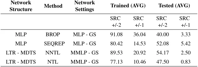
rela-Table 6.Comparison of average performances of MLP neural networks trained using tra-ditional Back Propagation and Method of Sequential Repetition with Progressive Action Development based on MLP Good Settings parameters and LTR – MDTS neural networks trained using NNTL and NTL Back Propagation algorithm based on Modified MLP Good Settings parameters
Network
Structure Method
Network
Settings Trained (AVG) Tested (AVG)
SRC +/-2
SRC +/-1
SRC +/-2
SRC +/-1
MLP BROP MLP - GS 91.08 36.04 40.00 3.33
MLP SEQREP MLP - GS 80.42 14.53 52.08 5.42
LTR - MDTS NNTL MMLP - GS 89.53 20.92 54.17 2.50
LTR - MDTS NTL MMLP - GS 77.13 10.46 47.50 0.83
tively similar results when rated with strict SRC criteria, here, for neural networks with LTR – MDTS neural network structure an emphasis is made towards neural networks that show better results regarding training set.
From the aspect of LTR – MDTS neural networks that are trained using NTL Back Propagation algorithm and Modified MLP Good Settings parameter values, when we con-sider weaker SRC criterion, the best results are obtained with neural network ann58_mdts that has 4 hidden layers with values of 83.72% on training and 55.00% on the test set. When we consider a strict SRC criterion, best results provides same neural network ann80_mdts with values of 16.27% for training and 5.00% on the test set.
Having in mind previously stated results from Table 6 it can be concluded that on the basis of SRC criteria LTR – MDTS neural network structure seems to be more suited for solving a presented problem when compared to traditional MLP neural network structure. However, on the basis of LTR – MDTS neural network structure, it can be concluded that neural networks that are trained using NTL Back Propagation in combination with Modified MLP Good Settings parameter values produce worse results than LTR – MDTS neural network that are trained with NNTL Back Propagation algorithm based on the same Modified MLP Good Settings parameter values.
Furthermore, having in mind that during training of neural networks with LTR – MDTS structure Modified MLP Good Settings parameter values, that are based on MLP Good Settings parameter values were used, it was decided to check if used parameters were actually the best parameters for LTR – MDTS structure. To confirm the above as-sumption, a series of tests was realized in order to track the impact of changes in the values of Learning Rate and Momentum parameters.
and 0.6, as for higher values of selected values are 0.8 and 0.9. In order to, reduce the influence of neuron random weight initialization as much as possible, it was decided that each neural network configuration will be trained 10 times from scratch, with a change of only one parameter value, in this case Learning Rate or Momentum, and to monitor deviations from the average value of the initial results. On the basis of relation of tracking parameter values against initial parameter value, two monitoring directions were formed that will track the impact of changes in the value of the parameter - increases (Up) and decreases (Down). Values that are higher compared to the initial value are marked as Up, while values that are lower than initial values are marked Down. With this test, for each best selected neural network regarding its class, 80 neural networks per neural network configuration were obtained, resulting in 480 trained neural networks with different train-ing parameter values.
By analyzing obtained results from conducted test, we have concluded that by de-creasing values for Learning Rate and Momentum parameters, performances of LTR – MDTS neural networks, could be improved up to a certain point. It is only needed to find appropriate ones. However, obtained results are considered to be worse than expected, therefore, it was concluded that by fine adjustments of training parameters, desired per-formance increase could not be obtained. Therefore, through "ad-hoc" methods of trial and error, several training settings combinations were tested until we determined training settings that are currently considered adequate for LTR - MDTS network and therefore are called LTR – MDTS Good Settings.
Good Settings parameter values that were used for training of LTR - MDTS neural networks are:
• Learning rate : 0.08 • Momentum : 0.1
Appointed parameters have been tested in combination with NNTL Back Propagation algorithm as well as in combination with NNTL Back Propagation algorithm. Results of aforementioned tests are presented in Table 7. Also, in Table 7, regarding values in column Network Settings value, LTR – MDTS – GS indicates that neural network was strained using LTR – MDTS Good Settings parameter values.
Regarding LTR – MDTS neural networks that are trained using NNTL Back Propa-gation algorithm and LTR – MDTS Good Settings parameter values, when we consider weaker SRC criterion, the best results are obtained with neural network ann16_mdts that has 1 hidden layer with values of 95.34% on training and 60.00% on the test set. When we consider a strict SRC criterion, it is considered that the best results provides the neu-ral network ann17_mdts that has 2 hidden layers with values of 32.55% for training and 5.00% on the test set although neural network ann118_mdts with 8 hidden layers can also considered to be the best regarding aforementioned strict SRC criterion.
on training set and 80% on test set, yet it was not selected as the best one regarding SRC +/-2 criteria since other neural networks had shown better results on training set.
It is important to emphasize that certain neural networks with LTR – MDTS have shown results of 80% on test set while none of neural networks with MLP structure have reached aforementioned score.
Table 7.Comparison of average performances of MLP neural networks trained using tra-ditional Back Propagation and Method of Sequential Repetition with Progressive Action Development based on MLP Good Settings parameters and LTR – MDTS neural networks trained using NNTL and NTL Back Propagation algorithm based on LTR – MDTS Good Settings parameters
Network
Structure Method Network Settings Trained (AVG) Tested (AVG)
SRC +/-2
SRC +/-1
SRC +/-2
SRC +/-1
MLP BPROP MLP - GS 91.08 36.04 40.00 3.33
MLP SEQREP MLP - GS 80.42 14.53 52.08 5.42
LTR - MDTS NNTL LTR – MDTS - GS 91.08 24.03 61.67 5.00 LTR - MDTS NTL LTR – MDTS - GS 88.37 11.24 70.00 7.50
Based on data from Table 7, regarding weak SRC criteria, if we consider performances of LTR – MDTS neural networks that are trained using NNTL Back Propagation algo-rithm, it can be concluded that provided results are certainly better than results that MLP neural networks trained with traditional Back Propagation algorithm provide. Regarding strict SRC criteria, it can be noted that MLP neural networks that are trained using tradi-tional Back Propagation algorithm show better results regarding training set, while on the test set better results have been shown by LTR – MDTS neural networks. If we compare LTR – MDTS neural networks that are trained with NNTL Back Propagation algorithm with MLP neural networks that are trained using Method of Sequential Repetition with Progressive Action Development, it can be concluded that MLP neural networks produce slightly better results regarding test set and strict SRC criteria. However, those results are better only by 0.42% and could be considered quite similar. On the other hand, LTR – MDTS neural networks based on all other criteria that are being tracked produce signifi-cantly better results than aforementioned MLP neural networks. Here it could be said that with using LTR – MDTS neural network structures in combination with NTL Back Prop-agation algorithm, a similar effect is obtained such as when using MLP neural networks with Method of Sequential Repetition with Progressive Action development.
LTR – MDTS neural networks that are trained using NNTL Back Propagation algorithm, provide better results than LTR – MDTS neural networks that are trained using NTL Back Propagation algorithm.
Also, when we compare performances of LTR – MDTS neural networks that are trained using NTL Back Propagation algorithm with LTR – MDTS Good Settings pa-rameter values and Modified MLP Good Settings papa-rameter values, it can be concluded that NTL Back Propagation algorithm provides better results with LTR – MDTS Good Settings parameter values than with Modified MLP Good Settings parameter values.
7.
Conclusion
Presented LTR - MDTS neural network structure provides a better solution to a Multiple Dependent Time Series problem compared to a traditional MLP Back Propagation neural network which was, in this particular case implemented in AForge.NET framework. As we stated before, LTR - MDTS structure is not a structure that solves time series problems better in general, yet it shows good results only in the scope of the presented problem. How will LTR – MDTS structure behave in the same domain of similar problems, and whether it they are applicable to a wider range of problems that can be solved using time series, at this time, we are not able to tell because they have not been tested on problems from aforementioned domains.
Extensive detailed results and performance of LTR - MDTS neural networks have been presented in this paper, however it is important to emphasize certain conclusions:
• LTR - MDTS neural networks on the structural level of a neural network, replicate multiple dependent time series structure.
• LTR - MDTS neural networks are, due to certain sliced synapses, from the computa-tional aspect easier to train, and free from backward time lapse effects.
• LTR - MDTS neural networks seem to be more sensitive towards value changes of Learning Rate and Momentum parameters due to sliced synapses.
• Two algorithms for training neural networks with LTR – MDTS structure have been devised: NNTL Back Propagation and NTL Back Propagation algorithm, both based on traditional Back Propagation algorithm
• If we compare the LTR - MDTS structure with MLP structures terms of the number of neurons in the neural network, it can be said that in most cases LTR - MDTS structures, regardless of the number of hidden layers have a higher number of neurons compared to the MLP network.
• When comparing LTR – MDTS neural networks with traditional MLP neural net-works it was noted that LTR – MDTS neural netnet-works in general produce better results on test sets, while MLP networks can be on pair with LTR – MDTS neural networks regarding results obtained on training set.
• There are configurations of neural networks with LTR – MDTS structure that have, on the basis of weak SRC criteria, obtained marks of 80% on test set that none of neural networks with MLP structure have obtained.
aiming for. We assume that presented behavior is most likely influenced by a small train-ing set size so neural networks did not manage to generalize exact referee’s movements regarding ball movement on a basketball court. However, since that is not our primary goal, and primary method for neural network performance evaluation is not a SRC crite-ria but a slight alteration of simulation of human horizontal field of vision that is described in paper Pecev et al. [21], it has been shown that, regarding aforementioned simulation, provided neural networks produce satisfactory results.
One of further research goals is to build a larger training set based on basketball ac-tions that are consistent trough out entire European region, conduct retraining of previ-ously trained neural networks and examine how training set size influences performance of aforementioned neural network structures. One of early further research idea was to develop an extended neural network that could reason based on the inputs that explicitly present basketball players in game and improve reasoned patterns of previously trained neural networks. That idea was abandoned and replaced with a system for basketball ref-eree path correction that is implemented in addition to simulation of human horizontal field of vision since we gave primary accent to aforementioned method of neural network performance evaluation.
Acknowledgments.The work is partially supported by Ministry of Education and Science of the Republic of Serbia, through Project OI174023: "Intelligent techniques and their integration into wide-spectrum decision support".
References
1. Ivankovi´c Z, Rackovi´c M, Markoski B, Radosav D, Ivkovi´c M (2010) Appliance of Neural Networks in Basketball Scouting. Acta Polytechnica Hungarica 7(4) : 167 - 180
2. Wan E.A, Beaufays F, (1998) Diagrammatic Methods for Deriving and Relating Temporal Neu-ral Network Algorithms. Adaptive Processing of Sequences and Data Structures Lecture Notes in Computer Science Volume 1387, pp 63-98
3. Vintan, L, Gellert A, Petzold, J, Ungerer T (2004) Person Movement Prediction Using Neural Networks. In First Workshop on Modeling and Retrieval of Context, Ulm, Germany
4. Connor J.T, Martin R.D, (1994) Recurrent Neural Networks and Robust Time Series Prediction. IEEE Transactions on Neural Networks, 5(2) : 240 – 254
5. Ruta D, Gabrys B, (2007) Neural Network Ensembles for Time Series Prediction. International Joint Conference on Neural Networks 2007 (IJCNN 2007) pp 1204 – 1209
6. Zhang P.G (2003) Time series forecasting using a hybrid ARIMA and neural network model. Neurocomputing Volume 50, pp 159–175
7. Landassuri-Moreno V.M, Bullinaria J.A (2009) Neural network ensembles for time series fore-casting. In 11th Annual conference on Genetic and evolutionary computation 2009 (GECCO 2009), pp 1235 -1242
8. Zhang G.P, Berardi V.L (2001) Time series forecasting with neural network ensembles: an ap-plication for exchange rate prediction. Journal of the Operational Research Society Volume 52, pp 652 - 664
9. Giles C.L, Lawrence S, Tsoi A.C (2001) Noisy Time Series Prediction using Recurrent Neural Networks and Grammatical Inference. Machine Learning 44(1) : 161 - 183
11. Khashei M , Bijari M (2010) An artificial neural network (p, d, q) model for timeseries fore-casting. Expert Systems with Applications 37(1) : 479 – 489
12. Teo K.K, Wang L, Lin Z (2001) Wavelet Packet Multi-layer Perceptron for Chaotic Time Series Prediction: Effects of Weight Initialization. Computational Science - ICCS 2001 Lecture Notes in Computer Science Volume 2074, pp 310-317
13. Ons B.R, Trabelsi A (2003) Optimizing Multilayer Perceptrons for time series prediction. BESTMOD, ISG, Université de Tunis
14. Patra M, Chakraborty S, Ghosh D (2012) Optimized Neural Architecture for Time Series Pre-diction Using Raga Notes. Speech, Sound and Music Processing: Embracing Research in India Lecture Notes in Computer Science. Volume 7172, pp 26-33
15. Markoski B, Pecev P, Ratgeber L, Ivkovi´c M, Ivankovi´c Z. (2011) A New Approach to Decision Making in Basketball - BBFBR Program, Acta Polytechnica Hungarica 8(6) : 111 - 130 16. Ratgeber L, Markoski B, Pecev P, Lacmanovi´c D, Ivankovi´c Z (2013) Comparative Review of
Statistical Parameters for Men’s and Women’s Basketball Leagues in Serbia". Acta Polytechnica Hungarica 10(6) : 151 - 170
17. Ivankovi´c Z, Rackovi´c M, Ivkovi´c M (2014) Automatic player position detection in basketball games, Multimedia Tools and Applications 72 (3) : 2741-2767
18. Najim, S. A, Al-Omari Z. A. M., Said, S.M (2008) On the Application of Artificial Neural Net-work in Analyzing and Studying Daily Loads of Jordan Power System Plant. Computer Science and Information Systems, 5(1) : 127-136
19. Abuadlla, Y, Kvascev G, Gajin, S, Jovanovi´c Z. (2014) Flow-Based Anomaly Intrusion Detec-tion System Using Two Neural Network Stages. Computer Science and InformaDetec-tion Systems, 11 (2) : 601-622
20. Loeffelholz B, Bednar E, Bauer K.W (2009) Predicting NBA Games Using Neural Networks. Journal of Quantitative Analysis in Sports 5(1) : Article 7. DOI: 10.2202/1559-0410.115 21. Pecev, P., Rackovi´c, M. & Ivkovi´c, M., 2016. A system for deductive prediction and analysis of
movement of basketball referees. Multimedia Tools and Applications, DOI 10.1007/s11042-015-2938-1, 75 (23) : 16389 - 16416
22. Giles, M., 2015. https://people.maths.ox.ac.uk/gilesm/. [Online] Available at: https://people.maths.ox.ac.uk/gilesm/mc/mc/lec1.pdf [Accessed 5 January 2016].
23. Karmilasari, S. M., 2005. http://karmila.staff.gunadarma.ac.id/. [Online] Available at: http://karmila.staff.gunadarma.ac.id/Downloads/files/16687/Tayangan+Backpropagation.pdf [Accessed 4 August 2014].
24. Menon, A. R., Mehrotra, K., Mohan, C. K. & Ranka, S., 1994. Characterization of a Class of Sigmoid Functions with Applications to Neural Networks. Electrical Engineering and Computer Science Technical Reports, Paper 152, pp. 1-28.
25. Beiu, V., Peperstraete, J., Vandewalle, J. & Lauwereins , . R., 1994. Close Approximations of Sigmoid Functions by Sum of Steps for VLSI Implementation of Neural Networks. The Scientific Annals, Section: Informatics, 40(1), pp. 31-50.
Miloš Rackovi´c was born 25.12.1965. He received B.Sc. in 1989., M. Sc. in 1993. with a thesis “Construction of a Translator for the Robot-Oriented Programming Languages”, and Ph. D. in 1996, with a thesis “Generating of the Mathematical Models of Complex Robotic Mechanisms in Symbolic Form”. He is a full Professor since 2006, at Department of Mathematics and Informatics, Faculty of Sciences, University of Novi Sad. Works in computational science and his main research areas are the intelligent information systems, databases and artificial intelligence. Head of Bachelor studies in Informatics. He has been coordinator of one WUS project and participated in several other multilateral projects. Good interpersonal and communication skills and team spirit. Author or co-author of 5 textbooks and more than 100 research papers. He is member of Editorial Board of Computer Science and Information Systems Journal. Great experience in curricula and syllabi creation and developing of the Faculty information system (especially the student service subsystem).