Communication Mechanism and Experimental Research of Super-Low Frequency Mechanicanl Antenna Based on Rotating Permanent Magnet
Xiaoyu Wang1, Wenhou Zhang1, Xin Zhou1, Zhenxin Cao2 and Xin Quan2
1. College of Mechanical Engineering, Dalian Jiaotong University, Dalian 116045, China;
2. College of Information Science and Engineering, Southeast University, Nanjing 2111895, China;
* Corresponding author:Xiaoyu Wang (e-mail:[email protected])
This work was supported in part by the Equipment Pre-research Fund (No. 61405180302).
Abstract: Super-low frequency communication technology has a broad application prospect in submarine, mine emergency, earthquake prediction and military and other fields. Super-low
frequency mechanical antenna excites electromagnetic wave through the mechanical movement of permanent magnet, converts mechanical energy into electromagnetic energy, and realizes wireless
communication. Based on the theory of ampere-current, the analytical model of radiation field of a constant rotating permanent magnet is established by introducing the parameters of the permanent
magnet and the measured distance. The relationship between the influencing factors and the radiation field of rotating permanent magnet was studied experimentally. The propagation
characteristics in air, soil and sea water were studied by simulation, and communication experiments were carried out by using 2FSK signal modulation. The results of simulation and experiment show that the radiation intensity of axial rotating permanent magnet is higher than that
of radial rotating permanent magnet. Propagation losses increase in air, soil, and sea water. The radiation intensity of a rotating permanent magnet is proportional to its volume. Through the
real-time control of the speed, the signal is transformed in real-time-frequency domain to realize super-low frequency communication. The model can be used for size evaluation and optimization of
super-low frequency antenna.
Keywords: Antenna measurements, Antenna radiation patterns, Antenna theory, Communication system
reliability, Magnetic field measurement
1. Introduction
Super-low frequency (SLF) electromagnetic wave (30Hz~300Hz) has received much attention in recent years due to path loss is less in water and soil and strong anti-interference ability, which offer a whole new idea about antennas. Super-low frequency mechanical antenna (MA) is a novel low-frequency electromagnetic transmission technique which utilizes the mechanical motion of electric dipoles or magnetic dipoles to generate the electromagnetic wave directly [1-2]. It has possible uses in the shore to dive, navigation and positioning field and has also been investigated as a potential communication technology.
One way to generate the electromagnetic wave is to use magnetic/piezoelectric heterostructure.
For example, Simovski C et al. showed that have carried out asymmetric excitation on the piezoelectric film, and electromagnetic radiation is generated by symmetry breaking effect [3].
Tianxiang Nan et al. use magnetic/piezoelectric heterostructure to form magnetoele-ctric antenna and
produce high-frequency radiation field with small electrical size [4-8]. So that the size of antenna can
get rid of the dependence on wavelength. However, these novel technologies are applied to high frequency antennas and are not extended to SLF antennas. Therefore, in December 2016, the defense
advanced research projects agency (DARPA)'s office of Microsystems technology issued an interagency announcement, the A Mechanically Based Antenna (AMEBA) development project was
officially launched in August 2017 [9]. The main idea of this project is to generate SLF time-varying magnetic field by mechanically moving electrets or permanent magnets, and directly convert mechanical energy into electromagnetic energy without impedance matching.
For the transmitting module of SLF mechanical antenna, the electret has a high radiation efficiency compared with the permanent magnet under the same conditions. But there are technical
difficulties in generating stable, persistent and high-density static charge (10−6𝐶/𝑚2) on the electret.
Therefore, many researchers choose rotating permanent magnet as the scheme of transmitting
module of mechanical antenna [10]. Madanayake et al. proposed an underwater positioning system with at least three mechanical antennas as the reference point and a multidimensional vector
magnetometer as the receiver. They assuming that the time-varying magnetic field generated by the dipole has the same spatial distribution as that generated by the static dipole, the magnetic field equation of the mechanical rotating dipole was derived [11]. Srinivas Prasad M N et al. concluded
that a spinning magnet system is not affected by the Chu Harrington limit in SLF communications, and derived an equation for electromagnetic fields in the far field [12-13], but there is not study of
that in the near field properties. In fact, the radiation intensity of the rotating permanent magnet in the far field is so weak that it is difficult to detect and receive. Therefore, the near field propagation
characteristics of rotating permanent magnets may be a research focus.
For the receiving module of SLF mechanical antenna, magnetic strength measuring instruments
with pT resolution mainly include: search coil magnetometer and optical pump magnetometer, magnetometers with resolution of up to 10pT mainly include Giant Magneto Resisive(GMR) [14-15].
Srinivas Prasad M N et al measured the time-varying magnetic field of the rotating magnet array with an extremely low frequency ferrite antenna. They collected and analyzed magnetic field signals within a range of 3 meters to verify its feasibility for extremely low frequency communication [16].
Slawomir Tumanski analyzed the principle and characteristics of coil winding in different ways, and proposed a coil design and parameter optimization method that comprehensively considered the two
factors of SNR and sensitivity [17]. However, they only theoretical derivation, no experimental verification. Miaoyu Zhang et al. proposed a new two-transmit and one-receive common face array
structure to improve the SNR of the coil [18]. Martinez et al. studied the coil's equivalent inductance, equivalent resistance and equivalent capacitance at high frequency, and established a mathematical
model of the coil's geometric parameters and equivalent inductance, equivalent resistance and equivalent capacitance [19]. Hunter c. Burch et al designed a receiver consisting of a triaxial
orthogonal coil and a 24-bit audio data recording card. The positioning effect of the receiver was analyzed theoretically and experiment-tally, which proved to be feasible and practical when the frequency was lower than 500 Hz and the distance was over 100 meters [20], but the specific frequency
value of the acquisition signal cannot be determined.
The present paper presents a mechanism of mechanical antenna. Based on the equivalent motion
model of the magnetic dipole, the physical model of the mechanical antenna and the time-varying electromagnetic field distribution model generated in free space are established, and the basic
an analytical model of its radiation field was established by introducing the parameters: the residual
magnetism of the permanent magnet, the volume and the test distance of the permanent magnet. For the coil receiver, introduce parameters: coil diameter, coil side length and coil turns, and establish the
analytical model of coil sensitivity. The relationship between the influencing factors and the radiation field of rotating permanent magnet was studied experimentally. The correctness of the theoretical
model and the feasibility of the mechanical antenna are verified by experiments. Finally, through the experimental test of the mechanical antenna prototype based on the rotating permanent magnet, the loading of the near-region magnetic field information is verified and analyzed.
2. Theoretical model
Consistent with the traditional super-low frequency antenna, the super-low-frequency
mechanical antenna is divided into radiating unit and receiving unit. The information loading of the radiation unit is realized by the mechanical movement of the permanent magnet, that is, the
transmitted information is loaded into the mechanical movement of the mechanical antenna by the signal generator. In this state of motion, the radiation unit of the mechanical antenna only needs to
maintain or change the energy of its mechanical state of motion, and use less energy to generate super-low frequency electromagnetic wave to transmit the signal. The information collection of the receiving unit is realized by the induction of time-varying magnetic field by the magnetic sensor, that
is, the induction electromotive force is generated by the induction of time-varying magnetic field by the magnetic sensor. The oscilloscope converts the induction electromotive force signal into digital
and transmits it to the upper computer for communication.
2.1. Theoretical model of mechanical antenna transmitting unit
2.1.1. Radiation unit field source model
The main idea of the transmitting end of mechanical antenna is to generate SLF time-varying
magnetic field through the mechanical movement of electrets or permanent magnets and convert the mechanical energy into electromagnetic energy. Using coulomb's law, electret and cylindrical
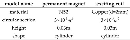
permanent magnet as excitation sources are equivalent to exciting coil and two charged surfaces. Calculate the conditions required to generate the same magnetic field intensity. The parameters of permanent magnet and exciting coil are shown in table 1.
Table 1. Parameter table of permanent magnet and exciting coil
model name permanent magnet exciting coil
material N52 Copper(d=2mm)
circular section -3 2
3 10 m 3 10 -3m2
height 0.03m 0.03m
shape cylinder cylinder
The model of permanent magnet and exciting coil is shown in figure 1. The magnetization
intensity of permanent magnet is
M
0=
1.1 10
6A m
/
. According to the equation (1), the coil generatesthe magnetic field intensity of H=1.1 10 6A m/ , which requires the excitation current of I=100A, and the number of turns of the exciting coil is N=330. However, the 12AWG coil can withstand a
functioning, the magnetic field intensity of the same size permanent magnet is higher than that of the
exciting coil. Therefore, this paper chooses rotating permanent magnet as the radiation unit of SLF mechanical antenna.
/ e
H= N I L
(1)
Where N is the number of turns of the exciting coil; H = N I L/ e is the excitation current; and
e
L is the effective magnetic circuit length of the exciting coil
I=12.5A
exciting coil N=330
3×10⁻³m2
N52
0
.03
m
permanent magnet
eight series connection
Figure 1. Model diagram of permanent magnet and exciting coil
2.1.2. Theoretical model of radiation element field intensity
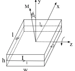
Rotating permanent magnet generates time-varying magnetic field in space, changing magnetic field induces changing electric field, and changing magnetic field and changing electric field are
coupled to form electromagnetic wave. As shown in Figure 2, in the cartesian coordinate system, the center point of the rectangular permanent magnet is taken as the origin. The permanent magnet rotates with the z-axis and at a constant angular velocity
. Rotation angle
0 is the included angleformed by the position of the initial magnetization direction of the permanent magnet and the
position of the magnetization direction after rotating about the z-axis.
z
w
l
x
y
M0
1
2 3
4
h
I
Figure 2. Diagram of rotating permanent magnet
According to ampere current model, the uniform magnetization of the permanent magnet is equivalent to the surface of the ampere current, current direction as shown in figure 2 arrow direction,
and equation for the equivalent surface current density α⃗⃗ is as follow
ˆ
M n
=
r
r
(2)Where Mr is the magnetization vector of magnetic body; and nˆ is the normal unit vector oriented from magnetic body to transmission medium.
Figure 2 shows the surface current is distributed on the magnetic pole surface of a cuboid parallel to the magnetization direction (four surfaces marked as 1,2,3,4 in figure 2), and there is no surface
The rotating permanent magnet as the transmitting end of the mechanical antenna, the
equivalent current is only distributed on its surface, and the retarded potential
A r t
r r
( )
,
is as follow( )
, ( ) ,4 t
R J r t
c
A r t ds
R − =
r r r r (3)Where,
is the permeability of the transmission medium; R is the distance between field pointrr and source point rr; c is the speed of light; ( )t is the integral domain (four sides of 1, 2, 3 and
4 marked in figure 2); and J r t, R
c −
r r
is the volume current density of source point rr at time
R t t
c = − .
For permanent magnets as shown in figure 2, the retarded potential
A r t
r r
( )
,
can be deduced as( )
0 ( )(
) (
) (
)
0 3 ˆ ˆ ˆ
, 1
4
j kr t
j e
A r t B Ve z x jy x jy z jkr
r − − = − + + + − r r (4)
Where B0 and V are respectively remanence and volume of the permanent magnet, and
0
B =
M; kc
= is wave number.
According to equation (3), shape parameters can be introduced into the integral region of permanent magnets of different shapes, so that they can be applied to permanent magnets of different
models. The value of shape parameters is shown in table 2. The equation of the delay potential of the permanent magnet is
( )
0 ( )(
) (
) (
)
0 3 ˆ ˆ ˆ
, 1
4
j kr t
j e
A r t B Ve z x jy x jy z jkr
r − − = − + + + − r r (5)
Table 2. Shape parameters of permanent magnet
Permanent magnet geometry Shape parameter value
rectangle 1
cylindrical 1.7725
Based on the retarded potential
A r t
r r
( )
,
and the ampere current model, the equations ofmagnetic induction intensity
B r t
r r
( )
,
and electric fieldE r t
r r
( )
,
of rotating permanent magnet at rras the radiation end of SLF mechanical antenna are obtained.
( )
( )
( )(
)
(
2 2)
( 0)2 2 2
0 3
, , =
ˆ
- 2 sin
ˆ 2 cos
ˆ[ 1 (2 ) ]
4 j r
j
k t
r j kr
j kr jk r e
B Ve
B r t A r t
jkr k r cos
r
− − = + + + − + − + + r rr r r
( )
( )
( )(
)
(
2 2)
2 ( 0)2 2
3
3
ˆ 2 sin 2
2
ˆ 2 2 cos
ˆ[ 2 ,
) ]
,
( =
2 4
j j kr t
j MVe
E r t B
r jkr
jkr k r e
j kr jk r cos r t
w r
−
−
−
+ − + +
+ − − −
= r
r r r r
(7)
Where is the polar angle, the included angle between the test point and the origin connection direction and the positive z-axis direction; and
is the azimuth, the included angle between the testpoint and the origin connection direction and the positive x axis direction;
=
is the waveimpedance of the transmission medium; is the permeability medium;
is the dielectricconstant of the medium.
2.1.3. Radiation characteristics of radiation unit
Figure 2 shows the material of the radiation unit rotating permanent magnet is Nd-Fe-B, whose grade is N52. The motor drives the permanent magnet at a speed of 4500r/min, and the operating
frequency of the electromagnetic wave emitted is 75Hz. The length, width and height of the permanent magnet are w=200mm, l=400mm and h=100mm, respectively, so the volume of the
permanent magnet is 8 10 −3m3. According to equation (6), the time-varying magnetic field intensity generated at 2.063km is 0.1pt. At present, the minimum magnetic induction intensity that can be detected by magnetic field measuring instruments on the market is 0.1pt.
When the propagation medium is air, it can be known from the equation (8) that, the corresponding wavelength is =4000km. Therefore, for rotating permanent magnet as the radiation
unit of mechanical antenna, its far field is difficult to measure. Therefore, it is more meaningful to study the near field of rotating permanent magnet.
c
f
= (8)
Where
f
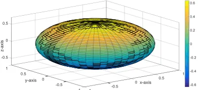
is the rotation frequency of the permanent magnetSimulating the traditional antenna pattern , and the radiation field pattern of the mechanical antenna radiating element was simulated by Maxwell. Select a standard spherical area with r=100m,
obtain the magnetic field strength on the standard spherical surface according to equation (6), divide by the maximum magnetic field strength on the spherical surface, and use the ratio to draw of the
mechanical antenna directional diagram through Matlab, as shown in Figure 3.
Figure 3. Direction diagram of rotating permanent magnet at near field
the z-axis direction, and its ratio is 2 / 5 . Therefore, the rotating permanent magnet is an omnidirectional antenna.
2.2. Theoretical model of mechanical antenna receiving unit
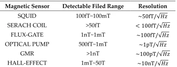
There are various kinds of magnetic sensors for magnetic field detection, and the detection range and resolution are shown in table 3. According to the equation (6), the time-varying magnetic field
strength of the rotating permanent magnet with volume of 1dm3 and remanence of 1T at 100m is
pT~nT. According to table 3, the optimal magnetic sensors for SLF time-varying magnetic field measurement are Superconduct Quantum Interfere Device (SQUID) and search coil. Although the
SQUID has a higher resolution than the search coil, and has good signal reception performance in table III, but it must work at a superconductor critical temperature close to 0K. While the mechanical
antenna used in military communications is usually operating at room temperature. Therefore, when using the superconducting quantum interferometer as the receiving antenna, the construction
environment is more demanding, while the receiving coil is simple in structure, convenient in construction and stable in performance. Therefore, the search coil is selected as the super-low
frequency receiving antenna in this paper.
3. A variety of typical magnetic sensor detection range and resolution table
Magnetic Sensor Detectable Filed Range Resolution
SQUID 100fT~100mT ~50fT/√𝐻𝑧
SERACH COIL >50fT < 100fT/√𝐻𝑧
FLUX-GATE 1nT~1mT ~100fT/√𝐻𝑧
OPTICAL PUMP 500fT~1mT ~1pT/√𝐻𝑧
GMR >1nT ~100pT/√𝐻𝑧
HALL-EFFECT 1mT~50T ~10nT/√𝐻𝑧
Sensitivity is an important index parameter for evaluating the receiving performance of the receiving coil, and its normalized model is conducive to the accurate design of the receiving coil.
Sensitivity evaluation is performed through an equivalent comparison of the antenna thermal noise voltage and the time-varying magnetic field induced voltage. Both the antenna thermal noise voltage and the time-varying magnetic field induced voltage are affected by the parameters of electrical
characteristics (equivalent resistance R, equivalent inductance L, equivalent capacitance C) of the coil.
In the SLF domain, the wavelength (103km~ 104km) of the electromagnetic wave is much larger than the width of the coil. Therefore, the winding capacitance and surface skin effect of the coil can be ignored. The receiving coil is an inductor composed of a coil, its equivalent circuit is shown in
figure 4. It consists of equivalent resistance R and equivalent inductance L.
R
L
V Ve
Figure 4. Equivalent circuit diagram of receiving coil
According to the definition of resistance, the coil resistance is equation (9)
1 2
4 Nc A
R
d
Where is coil resistivity; d is the wire diameter;
N
is the number of turns of the coil; A isthe cross-sectional area of the coil;
According to Biot-Savart Law, the inductance L of coils of various shapes can be obtained as
equation (10)
7 2 1
1 2
2 10 lnc A
L N c A c
N d
−
= −
(10)
Where c1 and c2 are coil shape coefficients, and coil coefficients of different shapes are shown
in table 4
Table 4. Coil shape coefficients of different shapes
Shape of coil c1 c2
square 4.000 1.217
equilateral triangle 4.559 1.561
right isosceles triangle 4.828 1.696
Based on the equations (9) and (10) [21], the parameters of electrical characteristics of the coil,
the equivalent resistance R and equivalent inductance L, are determined by three physical parameters of the coil, namely, coil turns number N, coil cross-sectional area A and single-turn coil diameter d. Therefore, deducing the relationship between the three coil physical parameters and the sensitivity S
is the key to the reasonable design of the receiving unit of the mechanical antenna.
In the SLF field, the wavelength of electromagnetic wave (4000km at 75Hz) is much larger than
the side length of the coil, so the radiation resistance of the coil can be ignored compared with the coil resistance. The minimum value of the detection signal is limited by the thermal noise generated
by the coil resistance R, The RMS of coil resistance R is its thermal noise voltage 𝑉𝑁𝑡 , and its
relationship is expressed as
4
Nt
V
=
KTR f
(11)Where K is boltzmann constant, Tis the absolute temperature (oK) of the conductor;
f
isthe noise bandwidth of the measurement system.
The coil sensitivity S is defined as the field equivalent of noise density, that is, the amplitude of
incident wave when the output voltage is equal to the RMS thermal noise voltage of the coil resistor R at the 1Hz bandwidth. Based on the time-varying field of the rotating permanent magnet, the
output voltage of the coil is shown in equation (12). Therefore, coil sensitivity S is equation (13).
( )
2 cos
a a a
V =
fN A B
(12)Where
f
is the working frequency of the rotating permanent magnet; is the includedAngle between the incident direction of time-varying magnetic field and the coil axis. When the coil axis is in the horizontal direction, it only represents the orientation of the receiver coil. Therefore,
( )
cos
in equation (13) can be ignored.4 2
KTR S
fNA
The sensitivity of the receiving antenna increases with the increase of frequency, but frequency
is an external factor affecting the sensitivity of the receiving antenna. In order to study the performance of different antennas, unifying the sensitivity calculation of different antennas, and the
sensitivity calculation equation of different antennas is expressed as
4 ˆ
2
KTR S
NA
= (14)
The equation of the sensitivity normalization shows that the measurement range of the sensitivity of the receiving coil can be improved by increasing the number of turns of the coil N and
the cross-sectional area A.
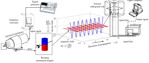
2.3. Mechanical antenna communication topology model
Since rotating permanent magnets are omnidirectional transmitting antennas. Based on the coil is most sensitive in its normal direction, a three-axis orthogonal coil is used to measure the
time-varying magnetic field in any direction in space. The time-time-varying magnetic field intensity is determined by the components in the three directions of x, y, and z using equation (15). Therefore,
the mechanical antenna communication topology model is shown in Figure 5.
2 2 2
x y z
B= B +B +B (15)
Where x, y , z and are time-varying magnetic field intensity values in three directions of space respectively; x direction is perpendicular to the rotation axis on the horizontal plane; The y direction
is in line with the rotation axis; z is the vertical direction
( ) 0 3
, = 4
B V B r t
r
(
)
3
,=
4
MV
E
r
t
r
magnetic field
e
le
c
tr
ic
f
ie
ld
Triaxial orthogonal coil
Upper computer
signal line
N
S
Rotating permanent magnet frequency
converter
drive input signal
Signal generator
oscilloscope
USB
signal line output signal
Figure 5. Mechanical antenna communication topology mode
Figure 5 shows the mechanical antenna communication topology structure. It is mainly divided into three parts, which are a radiating unit, a propagation path, and a receiving unit. The mechanical
antenna radiating unit transmits the signal to be transmitted to the frequency converter through a signal generator, and the frequency converter controls the rotation speed of the motor to drive the
permanent magnet to excite electromagnetic waves. The electromagnetic wave propagates in the air or the ground, and the induced electromotive force is generated by the time-varying magnetic field
induction through a three-axis orthogonal coil. The induced electromotive force is analog-to-digital signal converted by an oscilloscope. Then the digital signal is transmitted to the upper computer,
3. Simulated analysis
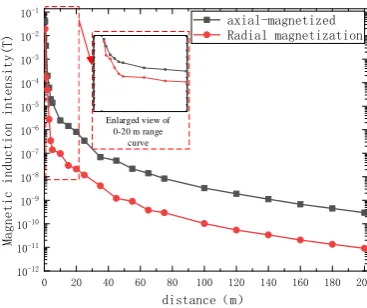
Permanent magnets are divided into axial magnetization and radial magnetization, the schematic diagram of which is shown in figure 6. The radiation field of a permanent magnet in space
varies with the direction of its magnetization. Therefore, the magnetic induction intensity of time-varying magnetic field of rotating permanent magnets with different magnetization directions will
also be different. Using the Maxwell to simulate the time-varying magnetic field generated by two rotating permanent magnets. Air is selected as the simulation propagation medium, and its detailed parameters and permanent magnet parameters are shown in table V. The change of magnetic
induction intensity with distance is obtained, and the result is shown in figure 7.
N
S
ω N
S
radially magnetized permanent magnet
axially magnetized permanent magnet
ω
Figure 6. Model of permanent magnet with different magnetization direction
0 20
1E-12 1E-11 1E-10 1E-9 1E-8 1E-7 1E-6 1E-5 1E-4 1E-3 0.01 0.1
Magnetic induction intensity(T)
distance(m)
axial-magnetized Radial magnetization
Enlarged view of 0-20 m range
curve
0 20 40 60 80 100 120 140 160 180 200
10-12
10-11
10-10
10-9
10-8
10-7
10-6
10-5
10-4
10-3
10-2
10-1
Magnetic induction intensity(T)
distance(m)
axial-magnetized Radial magnetization
Figure 7. Curve of magnetic induction intensity of rotating permanent magnet with distance
Figure 7 shows the radiation intensity of the rotating permanent magnet magnetized axially is higher than that of the radial permanent magnet. For rotating permanent magnets of the same volume
and material, the radiation intensity of the axial magnetized permanent magnet is about 15 times that of the radial magnetized permanent magnet. It can improve communication distance by nearly 2.5
times. Therefore, the radiation unit of the mechanical antenna chooses axial magnetized permanent magnet.
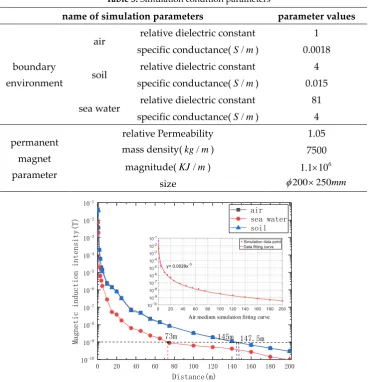
When rotating permanent magnets are used as radiation units of mechanical antenna, they are mainly used for propagation between air, sea and land. Therefore, the transmission medium of
mechanical antenna communication is mainly air, soil and seawater. In this paper, using the Maxwell to simulate the propagation characteristics of electromagnetic waves radiated by the rotating permanent magnet in air, seawater and soil, and the change of magnetic induction intensity with
distance was obtained. The properties of air, seawater and soil are shown in table 5. The result curve of time-varying magnetic induction intensity in the three media are shown in figure 8. Using the
Table 5. Simulation condition parameters
name of simulation parameters parameter values
boundary environment
air relative dielectric constant 1
specific conductance(S m/ ) 0.0018
soil relative dielectric constant 4
specific conductance(S m/ ) 0.015
sea water relative dielectric constant 81 specific conductance(S m/ ) 4
permanent
magnet parameter
relative Permeability 1.05
mass density(kg m/ ) 7500
magnitude(KJ m/ ) 6
1.1 10
size 200 250 mm
0 20 40 60 80 100 120 140 160 180 200 10-10
10-9
10-8
10-7
10-6
10-5
10-4
10-3
10-2
10-1
Magnetic induction intensity(T)
Distance(m)
air sea water soil
73m 145m 147.5m
Air medium simulation fitting curve
Figure 8. The change law of magnetic induction intensity of rotating permanent magnet
Figure 8 shows the radiation signal of rotating permanent magnet has the lowest propagation loss in air, followed by soil, and the highest loss in seawater. In the air and soil, the changing trend of
the time-varying magnetic field generated by rotating permanent magnets is basically the same. It is assumed that the minimum magnetic induction strength of the rotating permanent magnet can be
detected by the receiving antenna is 1nT. When the rotation frequency is 75Hz, the maximum communication distance are 147.5m in the air, 145m in the soil, and 73m in the sea water. In fact, some
SLF receivers can detect magnetic induction signals smaller than 1nT, so the communication distance will be longer. It can be seen from the fitting curve that the propagation medium is air that the
magnetic induction intensity is inversely proportional to the cubic of the distance. The mathematical model of rotating permanent magnet is proved to be correct.
4. Experimental verification
The influence factor of communication distance of mechanical antenna consists of two aspects:
radiation intensity of radiation unit and sensitivity of receiving antenna.
For the radiation unit, according to equation (6), the time-varying magnetic field intensity
and remanence of the permanent magnet. However, the materials limit the remanence number of
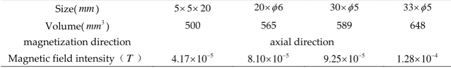
permanent magnet. So, increasing the volume of permanent magnet is the most effective way to improve communication distance. According to the simulation results, selecting 4 kinds of axial
magnetized permanent magnets, whose material is Nd-Fe-B and remanence is 1.38T. The detailed parameters are shown in table 6.
Table 6. Permanent magnet parameters and radition field intensity table
Size(
mm
) 5 5 20 206 305 335Volume(mm3) 500 565 589 648
magnetization direction axial direction
Magnetic field intensity(T) 5
4.17 10 − 5
8.10 10 − 5
9.25 10 − 4
1.28 10 −
For the receiving unit, according to equation (14), the sensitivity S of the receiving coil is mainly
affected by the number of turns N and the cross-sectional area A of the coil. The single factor analysis method was used to analyze the effect of coil turns N and cross-sectional area A on the sensitivity.
When studying the influence of coil cross-sectional area on coil sensitivity, coil 1 and 3 are designed
to fix other parameters and only change the coil cross-sectional area ( 2 2
0.36m →2.82m ). When
studying the influence of coil turns on coil sensitivity, coil 2 and 3 are designed so that other parameters are fixed and only coil turns (11→22) are changed. The detailed geometric parameters
of the coil are shown in table 7.
Table 7. EXPERIMENTAL COIL PARAMETERS
parameter coil 1 coil 2 coil 3
coil turns
N
21 11 21coil length of side(m) 0.6 1.68 1.68
Wire diameter(mm) 1 1 1
Coil Geometry square square square
Therefore, the influencing factors of the communication distance of the mechanical antenna are
the volume of the permanent magnet of the radiation unit, the number of turns of the receiving coil and the cross-sectional area of the receiving coil.
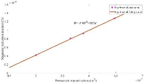
4.1. Influence of permanent magnet volume on communication distance
Figure 9 shows the motor drives the permanent magnet in table 6 at the speed of 4500rad/min to
excite the electromagnetic wave. Measuring the magnetic induction intensity at 10cm with a teslameter, obtain the magnetic field strength of the four permanent magnets. Using the Matlab to fit
the time-varying magnetic field intensity data generated by rotating permanent magnets according to equation (6), and the experimental fitting curve was obtained as shown in figure 10.
Replace 4 kinds of permanent
magnets
10cm
n=4500rad/min oscilloscope teslameter
Hall probe
Figure 10. Curve of relationship between volume and radiation intensity of rotating permanent magnet
Figure 10 shows the fitting curve is a linear equation curve about the volume of the permanent
magnet, whose intercept is not equal to 0. The reason why the intercept of the fitting curve is not equal to 0 is that there is an error in the measurement of the volume of the permanent magnet. The volume of permanent magnet is linearly related to the radiation intensity, which conforms to the
theoretical model of radiation intensity. With the increase of permanent magnet volume, the radiation intensity of rotating permanent magnet increases linearly. Therefore, the communication distance of
wireless electromagnetic wave can be improved by increasing the volume of rotating permanent magnet.
4.2. Influence of coil area on communication distance
As shown in figure 11, a is the signal generator and frequency converter, and b is the motor and
permanent magnet, which constitute the radiation unit. C is a three-axis orthogonal coil and d is an oscilloscope, which constitute a receiving unit. In the radiation unit, the permanent magnet driven by the motor excitations the electromagnetic wave, and its working frequency is 75Hz. The receiving
unit collects electromagnetic waves with the working frequency of 75Hz, and the communication distance is set as 6m. For the radiation unit, according to equation (6), the theoretical value of time-varying magnetic field strength generated at 6m on the rotating permanent magnet is 1.03
T .a b
c
d
Signal Input Device
B-Field Antenna
Signal Receiver
Analog to Digital Conversion
Computer
Figure 11. Photographs and block diagram of the mechanical antenna. (a)Signal input device, including signal
generator and frequency converte; (b) B-field divice, including motor, fixture and permanent magnet; (c) Signal
Table 8. Effective values of coil incluced voltage and tome-varying magnetic field strength
coils
Effective value of induced voltage/mV
Effective value of time-varying magnetic field
strength/T
Theoretical value of time-varying magnetic
field strength/T
Magnetic field strength
error/%
coil1 3.99 1.12
1.03
8.74
coil2 15.95 1.09 5.83
coil3 29.33 1.05 1.94
For the receiving unit, the three coils in table 7 were used to measure the time-varying magnetic field respectively to obtain its induced voltage time-domain diagram at 6m, and the
frequency-domain diagram was obtained by FFT transformation, as shown in figure 12. The effective values of induced voltage obtained from the time-domain diagram are shown in table 8. The time-domain
diagram shows that the operating frequency of time-varying magnetic field is 75Hz, which is the same as the rotation frequency of the motor. The effective values of induction voltage of each coil
were converted to the effective values of time-varying magnetic field strength and compared with the theoretical values. The results are shown in table 8.
0.00 0.02 0.04 0.06 0.08 0.10 0.12 0.14 0.16 0.18 0.20 0.22 -0.003 -0.002 -0.001 0.000 0.001 0.002 0.003 0.004 Induction electromoti ve force ( V )
Time(s)
coil 1
0.00 0.02 0.04 0.06 0.08 0.10 0.12 0.14 0.16 0.18 0.20 0.22 -0.04 -0.02 0.00 0.02 0.04 Induction electromoti ve force ( V )
Time(s)
coil2
0.00 0.02 0.04 0.06 0.08 0.10 0.12 0.14 0.16 0.18 0.20 0.22 -0.003 -0.002 -0.001 0.000 0.001 0.002 0.003 0.004 Induction electromoti ve force ( V )
Time(s)
coil3
50 60 70 80 90 100
0.00 2.50x10⁻⁶ 5.00x10⁻⁶ 7.50x10⁻⁶ 频率 振幅
50 60 70 80 90 100
0.0 3.0x10⁻⁶ 6.0x10⁻⁶ 9.0x10⁻⁶ 1.2x10⁻⁵ 1.5x10⁻⁵ 频率 振幅 0.006 0.012 -0.006 -0.012 -3
2.86 10
上峰值:
-3
-1.13 10
下峰值: -3 3. 99 10 -3
8.07 10
上峰值:
-3
-7.88 10
下峰值: -3 15 .9 5 10 6
5.05 10 @ 74.5 − Hz
5
1.13 10 @ 74.5 − Hz
0.032 0.024 0.016 0.008 0.000 -0.008 -0.016 -0.024 -3
20.41 10
上峰值: -3 2 9 .3 3 1 0 -3
-8.92 10
下峰值: 0.0050 60 70 80 90 100
2.50x10⁻⁵ 5.00x10⁻⁵ 7.50x10⁻⁵ 1.00x10⁻⁴ 频率 振幅 5
6.40 10 @ 75 − Hz
Down peak Up peak Down peak Up peak Down peak Up peak frequency am p li tu d e frequency am p li tu d e frequency am p li tu d e
Figure 12. FFT diagram of the signal the coil at 6mCommunication experiment
From the comparison between the experimental and theoretical values of coil 1 and coil 3 in table
8, it can be seen that when the cross-sectional area of the coil increases from 0.36m2 to 2.82m2, the measurement error of the same time-varying magnetic field decreases by 6.8%. By comparing the
experimental and theoretical values of coil 2 and 3, the number of coil turns increased from 11 to 21, and the time-varying magnetic field measurement error of the same target environment was reduced
by 3.89%. Therefore, the coil sensitivity can be improved by increasing the coil cross-sectional area and the number of turns. According to the frequency domain diagram of three kinds of coils in figure
its operating frequency is increased by increasing the number of turns of the coil. Therefore, the
communication distance of wireless electromagnetic wave can be improved by increasing the coil cross-sectional area and the number of turns.
4.3. Communication experiment
Antenna communication is the coupling between transmitting antenna and receiving antenna to
complete information exchange and transmission. The transmission signal after modulation, in the air and various media, its penetration is good, strong stability, signal is not easy to distortion, signal modulation usually adopts 2FSK modulation method. 2FSK is binary digital frequency modulation,
using of carrier frequencies to transmit digital information. The symbol ‘0’ corresponds to carrier frequency f1, and the symbol ‘1’ corresponds to the modulated waveform of carrier frequency f2,
and the change between f1 and f2 is instantaneous. When transmitting a ‘0’ signal, the carrier
whose transmission frequency is f1; When transmitting a ‘1’ signal, send a carrier with a frequency
of f2. Its working principle diagram is shown in figure 13.
Carr
ier
si
g
n
al
f
1
Carr
ier
si
g
n
al
f
2
2
FSK
s
ig
n
al
t
t
t
t
Bas
eb
an
d
s
ig
n
al
T 2T 3T 4T
0 1 0 1
Figure 13. 2FSK signal modulation schematic diagram
By simulating the signal modulation method of 2FSK , wireless communication experiment is
carried out on the mechanical antenna based on rotating permanent magnet, and the experimental facility is shown in figure 11.
The transmitted signal selects the square wave signal as shown in figure.14 (a). The input voltages of rotation frequency 0.5V and 1.6V are 60Hz and 200Hz respectively. Signal with a
frequency of 60Hz represents the carrier signal f1, and signal with a frequency of 200Hz represents
the carrier signal 𝑓2. When the motor receives the input square wave signal, it drives the permanent
magnet is 200Hz. From 2.00 to 4.00s, the input voltage of the motor is 0.5V, and the radiation field
frequency of the permanent magnet is 60Hz. These two waveforms correspond to the symbols 1 and 0 of the modulated signal respectively, processed by the short-time Fourier transform, and the result
is shown in figure 14 (c).
-4.8 -4.0 -3.2 -2.4 -1.6 -0.8 0.0 0.8 1.6 2.4 3.2 4.0 4.8
0 25 50 75 100 125 150 175 200 225 250 Fr equenc y(Hz) time(s)
-3.60 -3.24 -2.88 -2.52 -2.16 -1.80 -1.44 -1.08
-0.2 -0.1 0.0 0.1 0.2 0.3 0.4 Ma
gnetic induction intensity(T
)
time(s) Radiation field waveform
(a)
(b)
(c)
1 2 3 4 5 6 7 8 9 10 11 12
1 2 3 4 5 6 7 8 9 10 11 12
2.00 4.00
200Hz(f2) 60Hz(f1)
1 0 1 0 1 0
0
T 2T 3T 4T 5T 6T 7T time(s)
(d) B in a ry C o m m u n ic a ti o n si g n a l 0.50 1.00 1.50 2.00 in p u t si g n a l v o lt a g e (V ) 1.60 time(s)
Figure 14. Waveform of communication system (a) Input signal waveform; (b) Waveform of received signal
corresponding to frequency 𝑓1 and𝑓2 ; (c) Time domain diagram of received signal; (d) Transmission signal
waveform.
As shown in figure 14, the input signal waveform of the mechanical antenna communication system is basically the same as that of the output signal in time-frequency domain. As can be seen
from figure 14 (c), the graph of the short-time Fourier transform has a certain slope at the abrupt change in frequency. The reason for this phenomenon is that the motor needs a certain amount of
time in the process of changing the speed. Combined with the signal modulation method of 2FSK modulation principle, after the motor receives the square wave signal as shown in figure 14 (a), the
5. CONCLUSION
Traditional SLF antennas are bulky, power consuming and inefficient. This paper introduces a
kind of mechanical antenna with rotating permanent magnet as radiation element and triaxial orthogonal coil as receiving element. For radiation unit, a mathematical model based on rotating
permanent magnet and radiation field is established. For the receiving unit, a mathematical model based on the dimension parameters and sensitivity of the square coil is established. According to the analysis of theory, simulation and experimental results, some characteristics of the mechanical
antenna communication mechanism are obtained as follows:
(1) The radiation unit of the mechanical antenna is omnidirectional antenna;
(2) For the radiation unit of the mechanical antenna, the radiation intensity of the axial rotating
permanent magnet is about 15 times that of the radial rotating permanent magnet, and the
communication distance can be improved by about 2.5 times
(3) For the radiation unit of the mechanical antenna, the radiation intensity is proportional to the
volume of the permanent magnet and inversely proportional to the cubic of the test distance.
(4) For the receiving unit of the mechanical antenna, increasing the coil area can improve the
sensitivity of the receiving antenna, thus increasing the communication distance.
The communication experiment of mechanical antenna shows that the mechanical antenna can be used for wireless communication. In addition, 2FSK signal modulation can be realized through
real-time control of motor speed.
REFERENCE
1. Liu C , Zheng L G, Li Y P, “Study of ELF Electromagnetic Fields from a Submerged Horizontal
Electric Dipole Positioned in a Sea of Finite Depth,” IEEE International Symposium on Microwave, pp.
152-157, 2009.
2. Barr R, Ireland W , Smith M J, “ELF, VLF and LF Radiation from a Very Large Loop Antenna with a
Mountain Core,” Microwaves Antennas & Propagation Iee Proceedings H, vol. 140, no. 2, pp. 129-134, Feb. 1993.
3. Simovski C , Miroshnichenko A , Belov P, “Comment on "Electromagnetic Radiation under Explicit
Symmetry Breaking,” Physical Review Letters, vol. 114, no. 14, pp. 147701, Aug. 2015.
4. Nan T , Lin H , Gao Y, “Acoustically actuated ultra-compact NEMS magnetoelectric antennas,”.
Nature Communications, vol. 17, no. 8, pp. 296, Oct. 2017.
5. Yao Z , Wang Y E , Keller S, “Bulk Acoustic Wave-Mediated Multiferroic Antennas: Architecture and
Performance Bound,” IEEE Transactions on Antennas and Propagation, vol. 63, no. 8, pp. 3335-3344, Aug. 2015.
6. N.-N. Yang, X. Chen, Y.-J. Wang, “Magnetoelectric heterostructure and device application,” Acta
Physica Sinica, vol. 67, no.15, pp. 157508, Aug. 2018.
7. Bin Y , Zhong-Qiang H , Yu-Xin, “Recent progress of multiferroic magnetoelectric devices,” Acta
Physica Sinica, vol. 67, no.15, pp. 157507, Aug. 2018.
8. Mark A. Kemp, Matt Franzi, Andy Haase, “A high Q piezoelectric resonator as a portable VLF
transmitter,” Nature Communication, vol. 19, no. 2, pp. 1715, Apr. 2019.
9. Bickford J A, Duwel A E, Weinberg M S, “Performance of electrically small conventional and
10. Wei S , Qiang Z , Bin L, “Performance analysis of spinning magnet as mechanical antenna,” Acta
Physica Sinica, vol. 68, no. 18, pp. 188401, 2019.
11. Madanayake A, Choi S, Tarek M, “Energy-efficient ULF/VLF transmitters based on
mechanically-rotating dipoles,”Moratuwa Engineering Research Conference (MERCon). IEEE, pp.230-235, May. 2017.
12. Srinivas Prasad M N, Yikun Huang, Yuanxun Ethan Wang, “Going beyond Chu Harrington limit: ULF
radiation with a spinning magnet array,” IEEE International Symposium on Antennas and Propagation & USNC/URSI National Radio Science Meeting, vol. 32, pp.268-270, Aug. 2017.
13. Selvin S , Prasad M N S , Huang Y, “Spinning magnet antenna for VLF transmitting,” IEEE
International Symposium on Antennas and Propagation & USNC/URSI National Radio Science Meeting, vol. 32, pp. 1477-1478, Aug. 2017.
14. Mahdi A E , Panina L , Mapps D, “Some new horizons in magnetic sensing: high-Tc SQUIDs, GMR
and GMI materials,” Sensors and Actuators A (Physical), vol. 105, no. 3, pp. 271-285, Aug. 2003.
15. Pan Z, Zhou H, Zhang D, “Advances in detection circuit of magnetic sensors based on giant
magneto-impedance at abroad,” Chinese Journal of Scientific Instrument, vol. 38, no. 4, pp. 781-793, Apr.
2017.
16. Prasad M N S, Selvin S, Huang Y, “Directly Modulated Spinning Magnet Arrays for ULF
Communications” IEEE Radio and Wireless Symposium, vol. 1, no. 15,pp. 171-173, Jul. 2018.
17. Slawomir Tumanski, “Induction coil sensors—A review,” Measurement Sci & Tech, vol. 18, no.3, pp.
31-46, Jan. 2007.
18. Zhang Miaoyu, bao-long guo, Wu jie, “New coplanar coil system based on the tri-axial induction
logging,” Chinese Journal of Scientific Instrument, vol. 33, no. 5, pp. 170-178, May. 2018.
19. Martinez J L , Babic S , Akyel C, “On Evaluation of Inductance, DC Resistance, and Capacitance of
Coaxial Inductors at Low Frequencies,” IEEE Transactions on Magnetics, vol. 50, no. 7, pp. 1-12, Feb.
2014.
20. Hunter C. Burch, Alexandra Garraud, “Experimental Generation of ELF Radio Signals Using a