Spline Solution for a Fin with Temperature Dependent Thermal Conductivity

ISSN (online): 2349-784X

Spline Solution for a Fin with Temperature

Dependent Thermal Conductivity

Pinky Shah

Department of Mathematics V.N.S.G.U., Surat

Abstract

Fins are widely used to enhance heat transfer between primary surface and the environment in many industrial applications. Spline collocation method has been used to evaluate the efficiency of fins with temperature dependent thermal conductivity for exponential profile. The temperature distribution, fin efficiency and fin heat transfer rate are presented for exponential profile and a range of values of heat transfer rate are presented for exponential profile and a range of values of heat transfer parameters. The result reveal that spline solution is very effective and convenient, Comparison of the results DTM and Spline solution was shown that the analytical method and numerical data are in a good agreement with each other.

Keywords: Fins, Variable thermal conductivity, exponential profile, spline collocation method, heat transfer co-efficient _______________________________________________________________________________________________________

I. INTRODUCTION

Heat conduction analysis of fin is of great interest since they are used in many industrial applications such as air conditioning units, processor/ microprocessor cooling systems, refrigeration systems, heat exchangers, gas turbine blades and car radiators. The majority of the physical phenomena in the real world are described by nonlinear differential equations, where large class of these equations does not have analytical solution. The numerical methods are widely used in solving nonlinear equations.

The analysis of extended surface heat transfer is extensively presented by Kraus et at [1] Arslanturk[2] used decomposition method to evaluate the temperature distribution and analytical expression for the fin efficiency. Razelos and Imre [3] considered the variation of the convective heat transfer coefficient from the base of a convicting fin to its tip. A method of temperature-correlated profiles is used to obtain the solution of optimum convective fin when the thermal conductivity and heat transfer co-efficient are functions of temperature. Coskun and Atay [4, 5] used variation iteration method to analyze convective straight and radial fins with temperature dependent thermal conductivity. Sharqawy and Zubaie [6] carried out an analysis to study the efficiency of straight fins with different configurations when subjected to simultaneous heat and mass transfer mechanisms. Rajabi [7] obtained efficiency and fin temperature distribution by ADM and the HPM wit temperature dependent thermal conductivity. Lin and Lee [8] investigated boiling on a straight fin with linearly varying thermal conductivity.

Birkhoff[9] et al.worked on investigation of error bounds for spline interpolation 1964. Carl de Boor [10] was established the idea of existence and uniqueness of particular bicubic splines. Bickley [11] brought forward a useful aspect of spline functions in light that can be employed to solve a linear two point boundary value problem. Blue [12] the applicability of spline functions to nonlinear differential equations took place.

In this paper, we apply the application of the spline collocation method, to construct approximate solutions of the governing equations of the straight fins for exponential profile and temperature dependent thermal conductivity. This problem is compared with A. moradi and H. Ahmadikia [13].

Formulation of the Problem:

Consider a straight fin of the length L, with a cross-section area A x( ).Fin surface is exposed to a convective environment at temperatureT_. The local heat transfer coefficient h along the fin surface is constant, and the thermal conductivity varies with the temperature linearly. The one- dimensional energy equation can be expressed as:

   





0,

d dT

k T A x ph T T

dx dx

 

   

 

  (1) Where p is the periphery of the fin, T_ is the ambient temperature and k (T) is defined as





( ) _b 1 ,

k T k _ 



T T_ _ (2)

Where k_bis the fin thermal conductivity at ambient temperature and



is a constant.

( ) ( ),

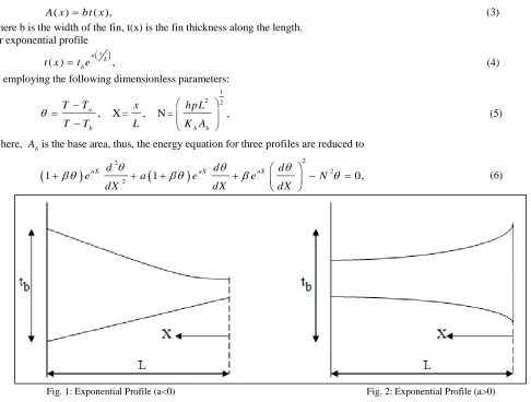
A x bt x (3) Where b is the width of the fin, t(x) is the fin thickness along the length.

For exponential profile

 

( ) ,

x a

L b

t x  t e (4) By employing the following dimensionless parameters:

1 2 2

, X = , N = ,

b b b

T T x hpL

T T L K A

 _    

 

 _{ } (5)

Where, A_bis the base area, thus, the energy equation for three profiles are reduced to









2 2

2 2

1 eaX d a 1 eaX d eaX d N 0,

dX dX dX

  

     

    _{ }  

  (6)

Fig. 1: Exponential Profile (a<0) Fig. 2: Exponential Profile (a>0)

Where,









T_bT_



in which T_bis the base temperature and fin tip is insulated. Therefore, boundary conditions for this problem are defined as follows:

0, =0,

x=1, =1.

x 

  

(7)

Basic principles of Spline Collocation

Use of Spline functions with moments for the solution of nonlinear differential equation was suggested by Blue [12]. Consider a linear two point boundary value problem

"( ) ( ) '( ) ( ) ( ) ( )

y x  p x y x q x y x  r x (8) Subject to the boundary conditions

 

1 ( ), '( ) 0

G y a y a  at xa

 

2 ( ), '( ) 0

G y b y b  at xb (9)

Since s(x) is a cubic Spline interpolating y(x) given by equation (6), we have s (xi) = y (xi), and also s"(x) is a linear function. Let us define this s"(x) in the subinterval [xi, xi+1] of [a, b] as follows:

" " 1 1

1 1

"( ) _i i _i i , 0,1, 2, .... 1

i i

x x x x

s x y y i n

h h

 

 

 

    (10)

Where h_i1 x_i1x_i

Two successive integrations produce a cubic Spline s(x) in [xi, xi+1] which has the form

 3  3    

" " 1 1

1

1 1 1 1

( )

6 6

i i i i

i i

i i i i

x x x x A x x B x x

s x y y

h h h h

 



   

   

    (11)

(IJSTE/ Volume 2 / Issue 10 / 223)

   

   

3 3 2

" " 1 1 "

1 1 1 2 " 1 1 1 1 1 ( )

6 6 6

6

i i i

i i i i

i i

i i i

i i

i i

x x x x h

s x y y y y

h h

x x h x x

y y h h                                 (12)

Similarly s(x) can be obtained in the interval [xi-1, xi] as

 3  3 2   2  

" 1 " " 1 "

1 1 1

( )

6 6 6 6

i i i i i i

i i i i i i

i i i i

x x x x h x x h x x

s x y y y y y y

h h h h

 

  

   

  _  _  _  _

    (13)

Deriving s'(x) at x = xi from the equation (13) which is denoted by s'(xi+), we have

" "

1 1 1

1

1

'( ) , 0,1, 2, .... 1

3 6

i i i i

i i i

i

h h y y

s x y y i n

h

  

 





      (14)

And in the same way

" " 1

1

'( ) , 1, 2, ....

6 3

i i i i

i i i

i

h h y y

s x y y i n

h



 



    (15)

Continuity of s"(x) at x = xi requires that s"(xi+) = s"(xi-)

So that " 1 " 1 "

1 ( 1) 1 1 1 1 1 , 1, 2, .... 1

6 6 6

i i i i

i i i i i i i i i i i i

h h h h

h y_  h h_ y h_ y_ h h_{ } y_    y   y_ _ i n

  (16)

This equation gives a system of (n-1) equations in (n+1) variables

y

_i

,

i



0,1, 2,...

n

to be determined. Therefore, the

moments

y

_i"

,

i



0,1, 2, ...n can be obtained from relation (15) if a curve is initially fitted to the data and two extra conditions are considered to complete the system. (16)

Here our objective is to solve the differential equation (6) with the help of relation (16). Let us express the equation (6) in the form

"( ) ( , , ')

y x  f x y y (17)

Subject to the boundary conditions (7) and (8). From these boundary conditions, it is seen that there are four pairs of boundary conditions as possible combinations viz.

1) y a( )K ; y b( )L 2) y a( )K ; y b'( )L 3) y a'( )K ; y b( )L 4) y a'( ) K ; y b'( ) L

The relation (16) will assumes the form for case (i) as









" " "

1 2 1 1 2 2

1 2 1 2 1 2 0 0 1 2

1 1 1 1

" " "

1 1 1

1 1

1 1 1 2

" "

1 1 1

2 1

6 6 3 6

( )

, 2 , 3, .... 1

6 6 3 6

6 6 3 6

i i i i i i i

i i i i i i

i i i

n n n n n n n

n n n n n n

n n

h h h h h h

h y h h y h y y y y

h y h h y h y

h h h h h h

y y y i n

h y h h y h y

h h h h h h

y y y

                                                     " n       (18)









2

" " 1

0 1 0 1 0

1 1 1 1

" " "

1 1 1

1 1

2

" "

2 1 2 1

2 "

6

( )

, 1, 2, 3, .... 1

6 6 3 6

2 4 "

6

i i i i i i i

i i i i i i

i i i

n

n n n n n n n

h

y y y y h y

h y h h y h y

h h h h h h

y y y i n

h

y y y y y h y

   

  

 

   



   

   



 

   

 

 

    

(19)

Similarly we are able to deal with remaining cases. It is observed for any case that on the left hand side the equations are obtained for which the coefficient matrix, for in the matrix form is upper tridiagonal one.

Now in order to obtain a solution to equation (16) with the boundary conditions given in equations (9), we fit a straight line y(x) = mx + c through the boundary points, which is of course an initial guess, the moments "

i

y

are calculated from the relation (12) at the nodal points x = xi as

" '

( , , )

i i i

y  f x y y For i = 0, 1, 2 ...n (20)

These moments are now utilized to evaluate yi, i = 0, 1, 2... n, through the relation (16) along with the two additional equations from boundary conditions. This can be furnished by solving merely a tridiagonal system of equations. The results so obtained can again be improve by continuing the same process till the desired solutions are found or two successive iterations produce the same values.

II. SOLUTION BY SPLINE COLLOCATION ITERATION METHOD Using equation (4) together with boundary conditions (5) are transformed into









2 2

2 2

1 eaX d a 1 eaX d eaX d N 0,

dX dX dX

  

     

    _{ }  

  (21)

The boundary conditions are 0, =0,

x=1, =1.

x 

  

(22)

For finding out the Spline approximation s(x) of ( )x described in equation (7) satisfying the boundary condition, a line

( )x ax b

   is assumed to be the first approximation to start with the iterative scheme. The straight line ( )x 1 can be fitted

through these points x=0 and x=1. The calculation of



_i, i = 0, 1, 2 ...N is to be carried out through the solution of tridiagonal system of (N+1) equations. The solution after obtaining the tridiagonal system of (N+1) equation is given below:

Table – 1

Comparison between Spline, exact and DTM results at  = 0 and N=1. x Spline Solution DTM Solution Exact Solution 0 0.78267298 0.78267175 0.78267175 0.1 0.78633413 0.78633664 0.786336641 0.2 0.79641962 0.796427754 0.796427754 0.3 0.81176472 0.81176631 0.81176631 0.4 0.831369483 0.831369483 0.831369483 0.5 0.854411785 0.85441111 0.85441111 0.6 0.880192387 0.880191752 0.880191752 0.7 0.908118163 0.908115721 0.908115721 0.8 0.937673562 0.937673304 0.937673304 0.9 0.968426627 0.968426886 0.968426886

(IJSTE/ Volume 2 / Issue 10 / 223)

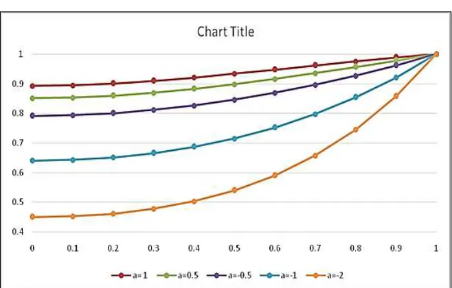
Fig. 3: Temperature Distribution of exponential profile (a=1) for different values of  at N=2

Fig. 4: Temperature profile fin for different values of N at =1.

III. RESULT AND DISCUSSION

The Comparison between the spline solution and DTM result for exponential profiles at = 0 and N=1 is shown in Table1. For assigned spline collocation results, Temperature distribution for different values of for N=1 is presented for exponential profiles in figure 3. Here, the spline solution results are compared to DTM while showing a good agreement between two methods.

There exists an indirect relation between the tip temperature rise and the values of N, because when N increases, the convective heat transfer rate increase, so those fins tip temperature decrease from figure 4.

From figure 5. From the result it can be concluded that, with decreasing , the fin base temperature decreases for exponential profile in straight fin.

IV. CONCLUSION

The spline collocation method was applied for solving heat conduction problem in the fin with different profiles and temperature-dependent thermal conductivity. This method supply reliable results in the form of numerical data and graph. Finally the heat transfer rate analyzed using this method and the effect of the fin parameter N and heat transfer parameters on dimension less temperature shown by figure. So spline collocation method has good approximation solution for the linear and nonlinear engineering problems.

REFERENCES

[1] A. Kraus, A.Aziz and J. Welty, Extended surface Heat Transfer, John Wiley and Sons, New York, NY,USA2001.

[2] C.Arslanturk, “A decomposition method for fin efficiency of convective straight fins with temperature-dependent thermal conductivity,” International communications in Heat and Mass Transfer, vol.32, no.6, pp.831-841, 2005

[3] P. Razelos, K.Imre, Journal of Heat Transfer 102(1980)420.

[4] S.B. Coskun and M.T. Atay,”Analysis of convective straight and radial fins with temperature-dependent thermal conductivity using variational iteration method with comparison with respect to finite element analysis,” mathematical Problems in Engineering, vol.2007,Article ID 42072,15 pages,2007. [5] S.B. Coskun and M.T. Atay,”Fin efficiency analysis of convective straight fins with temperature dependent thermal conductivity using variational iteration

method, “Applied thermal Engineering, vol. 28, no.17-18, pp.2345-2352, 2008.

[6] M.H. Sharqawy and s. M. Zubair, “Efficiency and optimization of straight fins with combined heat and mass transfer an analytic solution,” Applied thermal Engineering, vol. 28, no.17-18, pp.2279-2288, 2008.

[7] A. Rajabi homotopy perturbation method for fin efficiency of convective straight fins with temperature dependent thermal conductivity,” physics letters. Section a, vol.364, no. 1, pp. 33-37, 2007.

[8] W. W. Lin and D. J. Lee,” Boiling on a straight pin fin with variable thermal conductivity,” Heat and Mass transfer, vol. 34,no.5,pp.381-386,1999. [9] Birkhoff G. and Garabesian H., 1960 Smooth surface interpolation, J. Math. Phys., 39,258-268

[10] de Boor C.1962, Bicubic splines interpolation, J. Math. Phys., 41, 212-218.

[11] W. G. Bickley, “Piecewise cubic interpolation and two-point boundary problems,” The Computer Journal, vol. 11, pp. 206–208, 1968. [12] Blue J L (1969) Spline function methods for nonlinear boundary value problems, Communications of the ACM, 12(6), 327-330.