Spatial Density Voronoi Diagram and
Construction
Ye Zhao
Department of Mathematics and Physics, Shijiazhuang Tiedao University, Hebei Shijiazhuang 050043, China Email: [email protected]
Shujuan Liu and Youhui Zhang
College of Mathematics and Information Science, Hebei Normal University, Shijiazhuang, Hebei 050016, China Email: {[email protected], [email protected]}
Abstract—To fill a theory gap of Voronoi diagrams that there have been no reports of extended diagrams in spatial density so far. A new concept of spatial density Voronoi diagram was proposed. An important property was presented and proven. And a construction algorithm was presented. Spatial density can be used to indicate factors related to density such as conveyance and the traffic conditions. Some properties of spatial density Voronoi diagram were also introduced. In accordance with discrete construction method, achieved the construction of spatial density Voronoi diagram. Spatial density Voronoi diagram is a developed Voronoi diagram, and planar ordinary Voronoi diagram can be regarded as its special cases. It both perfected the theory about Voronoi diagrams, and extended the range of applications of Voronoi diagrams.
Index Terms—Voronoi diagram, Voronoi polygon, discrete, construction
I. INTRODUCTION
Voronoi diagram is one of a few truly interdisciplinary concepts with relevant material to be found in, but not limited to, anthropology, archaeology, astronomy, biology, cartography, chemistry, computational geometry, crystallography, ecology, forestry, geography, geology, linguistics, and urban and regional planning. An unfortunate consequence of this is that the material is extremely diffused, of varying mathematical sophistication and quite often idiosyncratic. The amount of material relating to Voronoi diagrams has also been growing steadily since the early 1980s .This proliferation results in part from the opening up of new areas of application and in part from the basic concept being extended in a variety of ways [1].
The concept of the Voronoi diagram is used extensively in a variety of disciplines and has independent roots in many of them. However, all kinds of Voronoi diagrams developed in Euclidean space. In fact, in many practical applications, the space is not ideal as Euclidean space. Spatial density also plays an important role. To take city Voronoi diagram for an example. The time from one point to another, relates either to the distance between the two points or the means of
conveyance and the traffic. The traditional Euclidean space could not indicate those important points [2].
To meet the practical requirement, this paper first mentioned the concept of spatial density Voronoi diagram. The concept represents population density, traffic conditions, climatic conditions and related factors. Spatial density Voronoi diagram perfects the theory about Voronoi diagrams, and the range of applications of Voronoi diagrams is extended. That makes great effort to the Voronoi diagram research and development.
II. PRELIMINARIES
In this section, we review briefly some notions and results related to Voronoi diagrams.
Definition 2.1 (a planar ordinary Voronoi diagram)
We consider a finite number, n, of points in the Euclidean plane, and assume that 2n. The n points are labeled by p1,p2,,pn with the Cartesian coordinates
x11,x12
,, xn1,xn2
or location vectorsn
x x
x1, 2,, . The n points are distinct in the sense that
j
i x
x for ij , i,jIn
1,2,,n
. Let p be an arbitrary point in the Euclidean plane with coordinates
x1,x2
or a location vector x. Then the Euclidean distance between p and pi is given by:
2 2 2 2 1 1,pi x xi x xi x xi
p
d
.
If pi is the nearest point from p or pi is one of the nearest points from p, we have the relation xxi xxj for
j
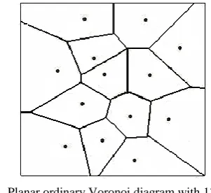
i , i,jIn. In this case, p is assigned to pi. Therefore, Definition 2.1 is written mathematically as follows. In the literature, a generator point is sometimes referred to as a site, as shown in Fig 1.
Definition 2.2 (a planar ordinary Voronoi diagram)
Let P
p1,p2,,pn
R2 , where 2n andxixj fori j, i,jIn. We call the region given by
pi
x x xi x xj for j i j In
V , (1)
the planar ordinary Voronoi polygon associated with pi (or the Voronoi polygon of pi), and the set given by
V=
V(p1),V(p2),,V(pn)
(2) the planar ordinary Voronoi diagram generated by P (or the Voronoi diagram of P). We call pi of V
pi thegenerator point or generator of the ith Voronoi polygon, and the set P
p1,p2,,pn
the generator set of the Voronoi diagram V (in the literature, a generator point is sometimes referred to as a site).Definition 2.3 (a planar ordinary Voronoi diagram defined with half planes)
Let P
p1,p2,,pn
R2 , where 2n andxixj fori j, i,jIn. We call the region
i I j j i i n p p H p V \ , (3)
the ordinary Voronoi polygon associated with pi and the set V(P)=
V(p1),V(p2),,V(pn)
the planar ordinary Voronoi diagram generated by P.The equivalence of Definition V3 to Definition V2 is
apparent, because xxi xxj if and only if
pi pj
H
x , for ji.
Definition 2.4 (an ordinary Voronoi diagram in Rm)
Let P
p1,p2,,pn
Rm, where 2n andj
i x
x forij, i,jIn. We call the region
pi
x x xi x xj for j i j In
V , (4)
i I j j i n p p H \ , (5)
the m-dimensional ordinary Voronoi polyhedron associated with pi , and the set V=
V(p1),V(p2),,V(pn)
the m-dimensional ordinary Voronoi diagram generated by P [3].Property 2.1 [4]
Let P
p1,p2,,pn
R2
2n
be a set of distinct points. The set V
pi defined by
pi
x x xi x xj for j i j In
V ,
A non-empty convex polygon, and V(P)=
V(p1),V(p2),,V(pn)
satisfies
2 1 R p V n i i
(6)
n j j i i I j i j i p V p V p V p V , , , \ \ . (7)
Property 2.2 [5]
For a Voronoi diagram generated by a set of distinct points P
p1,p2,,pn
R2
2n
, a Voronoi polygon V
pi is unbounded if and only ifp
i is on the boundary of the convex hull of P, i.e. piCH
P . Property 2.3 [6]For the Voronoi diagram generated by a set of distinct points P
p1,p2,,pn
2n
:(i) Voronoi edges are infinite straight lines if and only if P is collinear.
(ii) A Voronoi edge e(pi, pj) (≠Φ) is a half line if and only if P is noncollinear and pi and pj are consecutive generator points of the boundary of CH(P).
(iii) Suppose that pi and pj give a Voronoi edge e(pi, pj). Then this edge is a finite line segment if and only if
the line segment pipj is not an edge of CH(P).
Property 2.4 [7]
The nearest generator point of pi generates a Voronoi edge of V
pi .Property 2.5 [8]
The nearest generator point from pi exists in the generator points whose Voronoi polygons share the Voronoi edges of V
pi .Property 2.6 [9]
The generator pi is the nearest generator point from point p if and only if V
pi contains p.III. SPATIAL DENSITY VORONOI DIAGRAM
Definition 3.1 (spatial density distance)
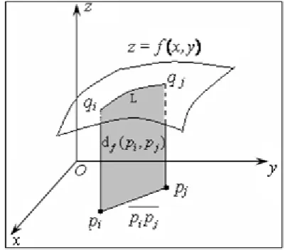
Given two arbitrary points pi, pj on a coordinate plane xOy, and z = f x, y( )0
is
a continuous function on the same plane. A plane through pi and pj is perpendicular to the xOy, and intersects surface z=f(x, y) at curve L. Points pi and pjare projections of qi and qj respectively on xOy, where qi and qj are two points on L. Then the region bounded by the points pi, pj, qi, qj and L is called the spatial density distance based on density distribution function z=f(x, y) in space, are denoted byd
f(
p
i,
p
j)
As fig. 2 shows, the shaded part is the the spatial density distance between points pi and pj based on density
distribution function z=f(x, y) in space.
Definition 3.2 (spatial density Voronoi diagram)
Let P
p1,p2,,pn
R2 , where 2n andxixj fori j, i,jIn. And distribution function z=f(x, y) is integrable in density space. We call the region
i j n i f i f if p pd p p d p p j i j I
V
, , , , (8)
the spatial density Voronoi polygon associated with pi based on density distribution function f (or the spatial density Voronoi polygon of pi), and the set given by:
Vorf=
Vf(p1),Vf(p2),,Vf(pn)
(9)the spatial density Voronoi diagram generated by P
based on density distribution function f (or the spatial density Voronoi diagram of P). We call pi of V
pi thegenerator point or generator of the ith spatial density Voronoi polygon, and the set P
p1,p2,,pn
the generator set of the spatial density Voronoi diagram. We call the set given by ( i) ( j)z z
i j
V p V p
spatial density
Voronoi edges. And points of intersection of the spatial density Voronoi edges are called spatial density Voronoi vertex.
Property 3.1
The planar ordinary Voronoi diagram is the generalization of the spatial density Voronoi diagram. Proof: When z = z x, y( )1, the value of spatial density distance
d
f(
p
i,
p
j)
is equal to that of Euclidean distanced(pi, pj). To wit df(pi, pj)= d(pi, pj)·1= d(pi, pj). Obviously, the Voronoi diagrams are same if they are based on the same distance. Thus, the planar ordinary Voronoi diagram is the particular case ( f=1) of the spatial density Voronoi diagram.
IV. DISCRETE CONSTRUCTION OF VORONOI DIAGRAM
Definition 4.1 (Discrete Distance) [10]
For each pixel p(x, y) on the screen, where 0xk,
l y
0 , x, y∈N, and k and l are the maximum value of abscissa and ordinate respectively. The distance between two pixels p1(x1,y1)and p2(x2,y2) are defined by
2 2 1 2 2 1 2
1, ) ( ) ( )
(p p x x y y
d (10)
Definition 4.2 (Discrete Voronoi diagram)[11]
LetP
p1,p2,,pn
, pi is the pixel on the screen,n
I
i . The region is
k j i j i p p d p p d p p d j i p p d p p d p p V k j i j i i n , , ) , ( ) , ( ) , ( ) , ( ) , ( ) ( (11)
the discrete Voronoi polygon associated with pi, and the set given by V=
Vn(p1),Vn(p2),,Vn(pn)
the discrete Voronoi diagram generated by P , and the set
p p pn
P 1, 2,, the generator set of the discrete Voronoi diagram.
Propertiy 4.1 ) ( )
( i n j
n p V p
V , for
i
j
.Propertiy 4.2
Discrete Voronoi edges are polygonal lines consist of pixels on screen.
Propertiy 4.3[12]
Discrete Voronoi regions consist of some pixel on screens, the distance from which to its generator less than that to the other generators. If there is a pixel that the
distance from it to its generator equal to that to another generator, the pixel is in the region of the generator which
has minor subscript values, as shown in Fig. 3. Figure 4. (a) The spatial density distance based
on density distribution function in space.
Figure 4 (b). Expanding centered on respective generators
Figure 4 (c). Judging before painting
Formaton of Discrete Voronoi Diagram [13]
Now we take 3 generator points as the example, and construct Voronoi diagram using discrete algorithm. First, we assign different colors for different generators, as shown in Fig. 4 (a).
Then expand centered on respective generators. In this process, every pixel we consider should be painted with the right color that is concordant with that of its generator, as shown in Fig. 4 (b).
Before paint every pixel, the color of the pixel should be judged. Only those pixels with white color are be painted. And if the pixel which is going to be painted is already a color one, proceed to next step, as shown in Fig. 4 (c).
The procedure end when all points on screen are marked color, as shown in Fig. 4 (d).
When all points on screen are marked color, the regions with different color form the Voronoi edges. To make the region boundaries visible, we do progressive scanning on full screen. Each time we record the color value of current pixel, and compare to the previous one. When two adjacent pixels are different color, one of them
is marked by black color (such as the first one is turned to black). The black pixels construct the Voronoi edges, as shown in Fig. 4 (e).
Do the second progressive scanning full screen. This time, we retain those black pixels, and turn other pixels to white color. Now we get the Voronoi diagram, as shown in Fig. 4 (f).
Fig. 4(a)-(f) gave a production process of Voronoi diagram with 3 generators, and the main technical steps of construction of Voronoi diagram are described in detail as following [14]:
Decision of Formation of Discrete Voronoi Diagram Region[15]
In programming, when all pixels of one Voronoi region associated with a generator point have already been marked, the generator point should be deleted from treating list consisted of set of generator point. The decision method is as following:
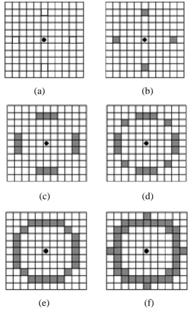
In the procession of expanding centered on respective generators, it is unable to form a circle for fixed radius value. Meanwhile, make radius value growing larger, repeat above procedure, and a closed circle may be formed. For a given generator point on screen, expand with a radius value r, there exists a minimum radius value e such that a closed circle be formed. And the expression
of r and e is: e2r22 r2 1. Figure 4 (e). Construction of the Voronoi
edges
Figure 4 (f). Voronoi diagram constructed with discrete algorithm.
(a) (b)
(c) (d)
(e) (f)
Fig. 5 shows the production process of a closed circle with r=4 and e=5.
Give n generator points on the screen, and expand centered on respective generators. In the process of painting, if there still white pixel, painted it with the right color, otherwise delete this generator point from treating list. Fig. 6 shows the judge processing, where the point p would be deleted.
Formation of Approximate Discrete Voronoi edges [16]
According to the actual requirement, we represent boundary with one color, and the background with another color. For instance, here we use black boundary and white background.
After scanning was over, all pixels on the screen are all marked color, as shown in Fig. 7 (a). First, we scan full screen from left to right. Each time we record the color value of current pixel, should compare with the previous one. If the two adjacent pixels are different color, the first one is marked black color, as shown in Fig. 7 (b). Then
scan full screen from up to down. If the two adjacent pixels are different color, the up one is marked black color. And Voronoi edges show up with black color. At last, do the third progressive scanning full screen. This time, we retain those black pixels, and turn other pixels to white color. Now we get the Voronoi diagram. Fig. 7
(a)-(d) shows the three times scanning full screen. (a) (b)
(c) (d)
Figure 6. Judge processing
Figure 7 (b). Scan screen from left to right
Figure 7 (c). Scan screen from up to down
Figure 7 (d). Scanning is over Figure 7. (a) All pixels on the screen
Algorithm of Discrete Voronoi Diagram [9]
Input:
p
1,
p
2,
,
p
n
, here,p
i is generator.Output: Voronoi diagrams generated by those generators. Step 1: Built linked lists L that holds generators’ data including: abscissa “x”, ordinate ”y”, power ”wi”, color Step 2: for generator, square of minor diameter “d2”, square of outside diameter “e2”;
Step 3: Initialize screen as white color; Step 4: Generate data sheet of Δx, Δy, and r2; Step 5: k=1;
Step 6: define a pointer to L;
Step 7: When is not empty, do loop: {( 1) Read data of row k: Δx, Δy, and r2; ( 2) read p->x, p->y, p->color;
{SetPixel (p->x+Δx, p->y, p->color); SetPixel (p->x-Δx, p->y, p->color); SetPixel (p->x , p->y+Δx, p->color); SetPixel (p->x , p->y-Δx, p->color);}
if one pixel above is black; then p->d2=r2;
else p->e2=r2; if p->e2 p->d2+2+1
then delete the node which “p” pointed to from L; if “p” point to the end of L
then k++, let “p” point to the first node of L; else p++;}
End.
V. CONSTRUCTION OF SPATIAL DENSITY VORONOI DIAGRAM
Fundamental Principle of Construction
According to the discrete method, scan the screen. And operation performed on each pixel point in a way that compute the spatial density distance between the pixel and each generator point denoted by d (f p p1, 2)
.
Thenjudge the pixel belongs to which Voronoi polygon. The spatial density Voronoi diagram form when scanning is over.
Particular way is: First, we assign different colors ci for each generator pi. Then scan the screen, deal with those pixel points qi, which still not be painted. If it belongs to the Voronoi polygon associated with pi, mark the pixel with the color of pi. When all points on screen are marked color, the regions with different color form the spatial density Voronoi edges. Then we can get the spatial density Voronoi diagram.
Algorithm of Spatial Density Voronoi Diagram
Input:
p
1,
p
2,
,
p
n
and spatial density function z=f(x, y), here, pi is generator.Output: Spatial density Voronoi diagrams generated by those generators based on density distribution function f. Step 1: Built array min[2] and array p- min[2];
Step 2: i=0, j=1;
Step 3: Compute the spatial density distance df(p, pi) between pixel which coordinates are (i, j) and its generator pi ;
Step 4: min[2]=min{ df(p, pi)}, p- min[2]= min{ df(p, pi)\ min[2]};
Step 5: When | min[0]- min[1]|<DELTA, do loop: {( 1) j=j+1;
if j≤YMAX; then turn to Step 4;
else turn to Step 7; ( 2) i=i+1;
if i≤XMAX; then turn to Step 3;
else End .
Application Models
Specific examples constructed by algorithm above-mentioned are as following:
Spatial density Voronoi with 300 generators which generate randomly based on density distribution function f=3(x+300) + 2 (y+500) is shown in Fig 8.
Figure 8. Spatial density Voronoi with 300 generators which generate randomly based on density distribution
function f=3(x+300) + 2 (y+500).
Figure 9. Spatial density Voronoi with 50 generators which generate randomly based on density distribution
function
9 144
2 2
y x
Spatial density Voronoi with 50 generators which generate randomly based on density distribution function
9 144
2
2 y
x
f is shown in Fig 9.
VI. CONCLUSION
A new concept and some properties of spatial density Voronoi diagram was proposed in this paper. The planar ordinary Voronoi diagram can be regarded as the generalization of the spatial density Voronoi diagram with the spatial density function f=1. Construction of spatial density Voronoi diagram is also presented and examples implementation is given in the end of the paper. Spatial density Voronoi diagram has better theoretical guiding significance and higher application values.
REFERENCES
[1] Pierre Alliez, David Cohen-Steiner, Olivier Devillers, Bruno Lévy, Mathieu Desbrun, Anisotropic polygonal remeshing, ACM Transactions on Graphics (TOG), v.22 n.3, July 2003.
[2] Jean-Daniel Boissonnat, Steve Oudot, Provably good sampling and meshing of Lipschitz surfaces, Proceedings of the twenty-second annual symposium on Computational geometry, June 05-07, 2006, Sedona, Arizona, USA. [3] Edetsbrunner H. Smooth surfaces for multiscale
shaperepresentation. In: Proceedings of the 15th Conference on Foundations of Software Technology and Theoretical Computer Science, Bangalore, 1995, pp: 391-412.
[4] David Bommes , Henrik Zimmer , Leif Kobbelt, Mixed-integer quadrangulation, ACM Transactions on Graphics (TOG), v.28 n.3, August 2009.
[5] Yang Liu , Wenping Wang , Bruno Lévy , Feng Sun , Dong-Ming Yan , Lin Lu , Chenglei Yang, On centroidal voronoi tessellation—energy smoothness and fast computation, ACM Transactions on Graphics (TOG), v.28 n.4, pp: 1-17, August 2009.
[6] Jane Tournois, Camille Wormser, Pierre Alliez, Mathieu Desbrun, Interleaving Delaunay refinement and optimization for practical isotropic tetrahedron mesh generation, ACM Transactions on Graphics (TOG), v.28 n.3, August 2009.
[7] Vyas, V., and Shimada, K. 2009. Tensor-guided hex-dominant mesh generation with targeted all-hex regions. In 18th International Meshing Roundtable conference proceedings.
[8] Yan, D.-M., Lévy, B., Liu, Y., Sun, F., and Wang, W. 2009. Isotropic remeshing with fast and exact computation of restricted Voronoi diagram. Computer Graphics Forum 28, 5, pp: 1445--1454.
[9] D. Micciancio and P. Voulgaris. Faster exponential time algorithms for the shortest vector problem. In Proceedings of SODA 2010. ACM/SIAM, Jan. 2010.
[10]M. D. Sikirić, A. Schürmann, and F. Vallentin. Complexity and algorithms for computing Voronoi cells of lattices. Mathematics of Computation, 78(267), pp: 1713--1731, July 2009.
[11]Naftali Sommer , Meir Feder , Ofir Shalvi, Finding the Closest Lattice Point by Iterative Slicing, SIAM Journal on Discrete Mathematics, v.23 n.2, pp: 715-731, June 2009. [12]Ye Zhao, Yajing Zhang. Dynamic construction of voronoi
diagram for figures. Proceeding 2009 IEEE 10th International Conference on Computer-Aided Industrial Design & Conceptual Design: E-Business, Creative Design, Manufacturing- CAID & CD 2009, 26-29, pp: 2189–2192. [13]Ye Zhao, Shu-juan Liu, Yi-li Tan. Discrete construction of order-k voronoi diagram. ICICA'10 Proceedings of the First international conference on Information computing and applications Springer-Verlag Berlin, Heidelberg 2010, pp: 79-85.
[14]Ye Zhao, Ya-Jing Zhang, Qing-Hong Zhang: Discrete construction of Voronoi diagrams for cross generators. 2010 International Conference on Machine Learning and Cybernetics, ICMLC 2010, 3, pp: 1556-1559.
[15]Ya-Jing Zhang, Ye Zhao, Jing Zhou, Xue-Fei Li, Jun-Jian Qiao. Optimum location on fuzzy clustering method. 2010 International Conference on Machine Learning and Cybernetics, ICMLC 2010, 4, .pp: 2094-2098.
[16]Wu Ran,Ye Zhao. Discrete Construction of Network Voronoi Diagram. ICMCI'2010, pp: 630-632.