On-line NNAC for a Balancing Two-Wheeled
Robot Using Feedback-Error-Learning on the
Neurophysiological Mechanism
Xiaogang Ruan
School of Electronic Information and Control Engineering, Beijing, China Email: [email protected]
Jing Chen (corresponding author)
School of Electronic Information and Control Engineering, Beijing, China Email: [email protected]
Abstract—A biomimic control structure is designed based on the sensorimotor system and the central nervous system of human brain. The main control center is focus on the cerebellar cortex functioning in supervised training. And then a method based on cerebellar model with feedback-error-learning on the neurophysiological mechanism was proposed to control a balancing two-wheeled robot which is a bionic self-balancing plant imitating human body. The cerebellar cortex as a forward controller was an on-line neural network adaptive controller and reflected the cerebellar function in balancing control problem. From the simulation including balancing control experiment, disturb experiment and mass changed experiment, we can see that the robot can be balanced in fixed position well by the biomimic control structure, and get a better result comparing the traditional feedback control.
Index Terms—Balancing Two-Wheeled Robot; balancing
control; sensorimotor system; feedback-error-learning; cerebellar internal model
I. INTRODUCTION
There are many kinds of two-wheeled self-balancing robot, such as wheeled-inverted pendulum, self-balancing wheelchair, JOE, nBot[1 ][ 2 ][ 3 ][ 4 ], and so on. All of them have ability of keeping balanced themselves and running forward. Many researches [3][ 5 ][ 6 ] on the balancing control are done after decoupling. Essentially, it is a kind of control method based on linear inverted pendulum. A lot of work has been done for such an inverted pendulum system. An adaptive output recurrent cerebellar model articulation controller is utilized to control wheeled inverted pendulums (WIPs)[7]. A mobile robot in [8 ] was controlled using a trajectory tracking algorithm based on a linear statespace model. Grasser et al. [3] developed a dynamic model for designing a mobile inverted pendulum controller using a Newtonian approach and linearization method. In [1], a dynamic model of aWIP was created with wheel motor torques as input, accounting for nonholonomic no-slip constraints. Vehicle pitch and position were stabilized using two controllers. Jung and Kim [9] created a mobile inverted
pendulum using neural network (NN) control combined with a proportional-integral-derivative controller. However, the balancing two-wheeled robot is a kind of MIMO nonlinear system, so the research on the control of MIMO nonlinear system is very important to robot control field.
In 1987, Kawato [10] proposed the inverse model and then proposed feedback error learning model [11] [12], which was designed from a biological perspective to establish a computational model of the cerebellum for learning motor control with internal models in the central nervous system. The error between expected and actual track was taken as the training signal, at the same time it solved the problem of normalization with different error information. As Kawato’s opinion, forward internal model predicts the action sequence and correspond with feedback control, which can overcome the time delay. Reference [13] present some theoretical investigations of the technique of feedback error learning (FEL) from the viewpoint of adaptive control, and prove its stability for SISO control system. Based on the balancing control of nonlinear system, in the year 2007, an on-line adaptive control for balancing based on feedback-error-learning scheme was proposed successfully into the inverted pendulum balancing control. To some extent, this learning scheme shows the function of cerebellum in keeping body balancing.
As we all know, in the nerve system, motor nervous system is for the motion and posture control. Our robot is designed imitating human, while cerebellum takes part in the balancing control. Therefore, it is very important to research the balancing control of robot according to cerebellar balancing control principle in the sensorimotor system, and there is important theoretical and practical value, especially for the human-simulated intelligent control (SHIC).
bionic control structure simulating the sensorimotor system is introduced. In Section Ⅳ, the feedback-error-learning algorithm is proposed with the cerebellar cortex as the adaptive neural network, and the on-line learning process is proposed for the continuous MIMO two-wheeled robot. The simulation experiment has been done for the balancing control with fixed-point using the method proposed in this section, and the comparative experiments with traditional feedback control method have been done. At the same time, experiment with step disturb has been made. Finally, the article comes to a conclusion in Section V.
II. SENSORIMOTOR SYSTEM
A. Central Nervous System
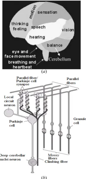
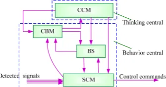
An important feature of the Central Nervous System (CNS) is its remarkable ability to adapt to changes both in the environment and inside the body. Motor nervous system includes motor center (MC) and PNS (Peripheral Nervous System). The whole nervous system can also be called sensorimotor nervous system. Motor nervous system is composed of three-level hierarchical structure and two auxiliary monitor systems. From low to high the three-level hierarchical structure is respectively the spinal cord (SC), brainstem (BS) and cerebral cortex (CC), while two auxiliary monitor systems mainly are the cerebellum and ganglion nuclear group in the forebrain area as the core. These brain areas related to motor control form interconnected circuit, and deal with all kinds of information processing of motion and postures. Figure 1(a) shows the regulation and control mode of behavior central; Figure 1(b) shows the global network of central nervous system linking the cerebellum, the basal ganglia and the cerebral cortex. the CB, the BG, and the CC exist for different types of learning.
Figure 1
Figure 2
(a) regulation and control mode of behavior central; (b) The global network of central nervous system linking the cerebellum, the basal ganglia and the cerebral cortex. CCM, cerebral cortex model; CB, cerebellum; BS, brainstem; SCM, spinal cord model
During the course of sensorimotor learning, the cerebral cortex(CC), basal ganglia(BG) and cerebellum(CB) work in parallel but particular ways [14][15][16]. The loop through the basal ganglia learns to discover ballpark actions that are appropriate in a given context [17], utilizing reinforcement learning. The loop through the cerebellum learns to refine the action through supervised learning. The cerebral cortex, driven by input from basal ganglia and cerebellum, learns through practice to perform these operations faster and more accurately, utilizing unsupervised Hebbian learning. The coordination of these diverse forms of learning has been simulated by Doya[15].
B. Cerebellum Internal Model
Along with the development of medical science, the research about brain structure is very mature to some extent. Figure 2(a) shows that the function of brain contains thinking, feeling, hearing, speech, motion, sensation, vision, balance and so on. Brain is the place of advanced nerve centre and controls these actions of human being. Thereinto, the cerebellar part mainly realizes the balance control of body. So that it is inevitable to design the balance system of robot using the cerebellar model mechanism in the research of bionic intelligent control. Figure 2 (b) exhibits the structure of cerebellum.
Cerebellum (a)
(b)
(a) structure of brain (b) structure of cerebellum
other part of brain for regulating and controlling the behavior.
In 1960s, many researchers (such as Brindley ) in the field of neurophysiology proposed that if synapse connection between parallel fibre and Purkinje cell could be amended, memory would be shaped. In the year 1968, Flourens became aware of the dynamic function of cerebellum. He pointed out that the function of cerebellum is to coordinate motion. For motion cerebellum is not necessary, but if there was no cerebellum, limb motion would became jerky, trembling, loose and imprecise. Ito [ 18 ] brought the concept of internal model into neurophysiology and proposed that internal model is the result of learning or conditioning. Basal ganglia used internal model to carry out motion control. And he pointed out the hypothesis of forward model. The disadvantage is that the feedback gain of forward model is small but the feedback delay is great, so it is difficult to realize the motion control depending only on forward model for basal ganglia organization. It makes against the rapid and steady of the motion control. The cerebellum is known to be critical for accurate adaptive control and motor learning.
Figure 4
Figure 3
III.
Regulate and control mode of behavior central with cerebellar model. CCM, cerebral cortex model; CBM, cerebellar model; BS, brainstem; SCM, spinal cord model
TWO-WHEELED ROBOT SELF-BALANCING
PROBLEM
A. B-TWR System Description
Here we study the B-TWR with two control inputs, which are the torques of the two wheels. And the system degree of the freedom is three, which is more than the control inputs. So the system belongs to under-actuated system.
B-2WMR is a nonholonomic system, and here the rigid model is discussed, which has two coaxial driving wheels. And there is an internal body which can install some subsystems, such as controllers, sensors, etc. The internal body is said to be Intermediate Body (i.e. IB). The holistic physical framework is shown in Figure 4(left).
left: system whole structure; right: side elevation of robot after simplification
Definition of parameters and variables are all shown in Table I.
TABLE I
DEFINITION OF PARAMETERS
Parameter Unit Value
, l r
m m : the mass of
the left and the right wheel kg 1 M: the mass of the Intermediate Body kg 10
R: radius of wheel m 0.15
d: the distance between
the center point of two wheels m 0.44
1
L: the distance
between the barycentre of IB and O m 0.4 Jl= Jr= Jw : the moment of inertia of
(left and right wheel) about its axis kg·m2 1.125e-2 Jy: the moment of
inertia of the robot about the y –axis kg·m2 1.5417 Jz: the moment of
inertia of the IB about the z –axis kg·m2 0.5893 g: acceleration of gravity m/s2 9.8 ,
l r
μ μ :frictional coefficient of
two wheel with ground N·m/(rad/s) 10,10 w
μ : frictional coefficient of the wheel axis N·m/(rad/s) 1
xv position and velocity m and m/s var ,
b b
θ θ : the inclination angle and angle velocity of the Intermediate Body
rad and
rad/s var ,
θ θ: yaw angle and angle velocity of robot. rad and
rad/s var ,
r l
ϕ ϕ: rotary angle of the right and left
wheel. rad var
, l r
ω ω : rotary angle velocity of the right and
left wheel rad/s var
d
τ : the disturb put on the body of robot N.m var
l
τ : torque provided by left motor N.m [-5,5]
r
τ : torque provided by right motor N.m [-5,5]
B. B-TWR Mathematical Model
The math model of balancing two-wheeled robot has been built, and the correctness has been validated.
The dynamic model can be described as
( ) + ( , )= + d
M q q D q q Eτ u (1)
In this equation, M( )q ∈\n n× is the system inertial matrix, 1
( , )∈ n×
D q q \ is the Coriolis force and gravity matrix, is the input vector, is the transition matrix of the input vector. is the disturb put on the robot.
r
∈
τ \ E∈\n r×
1
r× = d∈
ω u \
where
11 12 13
21 22 23
31 32 33
( )
a a a
a a a
a a a
⎡ ⎤
⎢ ⎥
= ⎢ ⎥
⎢ ⎥
⎣ ⎦
M q ,
1
2
3
1 1
( , ) , 1 0 , , 0 1
d
l dl
r dr
d d d
τ
τ τ
τ τ
− −
⎡ ⎤ ⎡ ⎤ ⎡ ⎤
⎡ ⎤
⎢ ⎥ ⎢ ⎥ ⎢ ⎥
=⎢ ⎥ =⎢ ⎥ =⎢ ⎥ = ⎢ ⎥
⎣ ⎦
⎢ ⎥ ⎢ ⎥ ⎢ ⎥
⎣ ⎦ ⎣ ⎦ ⎣ ⎦
d
2
11 1 12 21 13 31 1
2
2 2 2 2
22 2 1
2
2 2 2
23 32 2 1
2
2 2 2 2
33 2 1
1
( ); co
2 1
( ) ( sin
4
1 ( sin )
4
1
( ) ( sin
4
y b
l w b z
b z
r w b z
a ML J a a a a ML R
R
a m R J MR ML J
d R
a a MR ML J
d
R
a m R J MR ML J
d
s
)
)
θ
θ
θ
θ
= + = = = =
= + + + +
= = − +
= + + + +
2 2
1 1sin 1 sin cos 2
( )
b b b
w l r
d MgL θ Mθ L θ θ μ θw b μ ϕ ϕ
= − − + −
+
2 2 2
2 1 1
2 2 2
3 1 1
1
( ) ( ) sin 2 sin 2
( )
1
( ) ( ) sin 2 sin 2
( )
l r b b b b
l w l w b
l r b b b b
r w r w b
R
d ML ML R
d
R
d ML ML R
d
ϕ ϕ θ θ θ θ
μ μ ϕ μ θ
ϕ ϕ θ θ θ θ
μ μ ϕ μ θ
= − −
+ −
= − − − +
+ −
+
b, ,l r
The model is different from others. The frictions of two wheels with ground and of the wheel axis are considered. It’s supposed that the two wheels are restricted by the restriction of the pure rolling.
q is the generalized coordinate of system, and can be defined as =(θ ϕ ϕ )T
d
τ
r
τ
q , is the disturb put on the
body of robot. are respectively the torque provided by the left and right motor. We choose the Maxon DC motor, and the torque is limited in the bound of ±5Nm owing to the performance of motor.
and
l
τ
The kinematics model of robot can be described as
[
]
[
]
1
cos 2
1
sin 2
( )
l r
l r
r l
x R
y R
R d
ϕ ϕ θ
ϕ ϕ θ
θ ϕ ϕ
⎧ = +
⎪ ⎪
⎪ = +
⎨ ⎪ ⎪
= −
⎪⎩
(2)
Where (x,y) denotes the position of robot in the Cartesian
coordinate, and is the yaw angle
velocity of robot.
( l r) / R
θ= ϕ ϕ − d
IV.
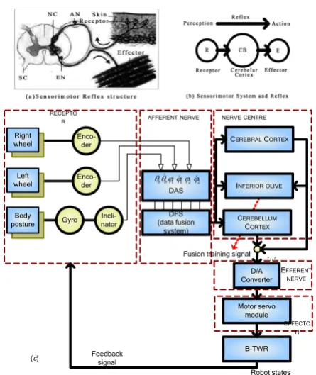
C. The bionic control structure
Simulating human brain structure, we form the bionic control structure as in Figure 5. For the sensorimotor, there are mainly five part including receptor, efferent nerve; central nervous; afferent nerve and effector. The on-line NNAC concentrates on the central nervous.
FEEDBACK ERROR LEARNING MODEL
A. Theoretical model with FEL
Supervised learning depends strongly on the availability of an external teacher. For a given set of inputs, neural network uses the error between the desired response from the teacher and the network’s actual output to adjust the interconnection weights between each
neuron. The whole control scheme is proposed in Figure 6.
Enco-der
DAS
DFS (data fusion
system) Left
wheel
Gyro Incli-nator
Body posture
Enco-der Right
wheel
1 1 2 2
b b θ θ ϕ ϕ ϕ ϕ
CEREBRAL CORTEX
CEREBELLUM
CORTEX
B-TWR INFERIOROLIVE
,
τ τl r
Motor servo module
D/A Converter
RECEPTO
R AFFERENTNERVE
EFFERENT NERVE
EFFECTO R NERVECENTRE
Fusion training signal
Robot states Feedback
signal (c)
Figure 5 Physiological principles of sensorimotor and the bionic control structure for B-TWR. SC, spinal cord; EN, efferent nerve; NC, central nervous; AN, afferent nerve; DAS, data acquisition system.
− 1( )
( )
n
e t e t#
fb
u
ff
u
e
Figure 6 NNAC based on feedback-error-learning scheme. MF, mossy fibres; GC, granule cells; PF, parallel fibres; PC, purkinje cells; CF, climbing fibres; IO, inferior olive;
As in literature [19], the NNAC is updated so as to realize the inverse model of controlled plant after learning. The parameter update law is
(
)
T
T
d
(1 ) d
ff
fb
u w
u k
t η w μ μ
∂
⎛ ⎞
= − ⎜ ⎟ + −
∂
⎝ ⎠ e (3)
where η is the learning rate of neural network and 0<η
<1, 0<µ<1, kT≥0. For the two wheeled robot system, we
have n1, r1, r1,
ff fb
u u k
× × ×
∈ ∈ ∈ ∈
e \ \ \ \n r× .
Therefore the aim of the training algorithm is to adjust the weights of the network so as to minimize the learning error:
T T T
1( (1 ) ) ( (1 ) 2 μufb μ k μufb μ
Ξ = + − e + − k e) (4)
For our robot, the cerebellar cortex network is designed with three layers. Input layer with six nerve cells, hidden layer with six nerve cells, and the output layer with two nerve cells which are the torques of two-wheels make up of the neural network.
B. On-line training algorithm for B-TWR
The proposed on-line training algorithm is given in Step 1 to Step 5:
ON-LINE TRAINING ALGORITHM
Step 1: Initialize the parameters: choose weights w0, bias weights b0 randomly, µ=0.56, η=0.5, k=[1,1,1,1,1,1;1,1,1,1,1,1]'.
Step 2: Repeat for each new input training pattern e and ufb.
Step 3: Calculate the parameter update law shown in formula (3).
Step 4: Update the weights according to the parameter update law.
Step 5: Calculate the output of the NNAC to control the robot.
The neural network can be expressed as follows:
6 1 6 6 6 1
1 1 1
6 1
1 1
2 1 2 6 6 1 2 1
2 2
2 1 2 1
2 2
tanh( )
N W b
A N
N W A b
A N
× × ×
× ×
× × × ×
× ×
⎧ = +
⎪ = ⎪ ⎨
= +
⎪
⎪ =
⎩
e 6 1
1 2
N1: the input of hidden layer
A1: the output of hidden layer
N2: the input of output layer
A2: the output of output layer
W1: the weights from input to hidden layer
b1: the bias weights of hidden layer
W2: the weights from hidden to output layer
b1: the bias weights of output layer
We can conclude formula (5) as in Appendix A.
(
)
(
)
T T
2
1
T 2
6 2 1
1 1 6
2 1
1 1 d
(1 )
d d
(1 )
d
d ( , ) (1 ( )) ( ) ( )
d d ( )
(1 ( )) ( )
d
( 1 6; 1 6)
fb fb
j
j
W
u k A
t
u k
t W i j
A j e i D j t
j
A j D j t
i j
η μ μ
η μ μ
η
η
=
=
⎧ = − + −
⎪ ⎪
⎪ = + −
⎪⎪ ⎨
⎪ = − −
⎪ ⎪
⎪ = −
⎪⎩
= =
∑
∑
e
b
e
b
" "
(5)
(
)
T T
2 fb (1 )
D W= μu + −μ k e
For our two-wheeled self-balancing robot, the varieties are following.
T
0 0 0 0 0 0
;
b b l r l r
l l r r
θ θ ω ω ϕ ϕ
ω ϕ ω ϕ
⎡ ⎤
=⎣ − − − − − − ⎦
= =
e
The initial incline angle is 9 degree(π/20 rad), and other variables are all zero.
Feedback controller is a feedback gain matrix: 100 40 1 4 0 3 K_back =
100 40 4 1 3 0
⎡ ⎤
⎢ ⎥
⎣ ⎦
C. Simulation Experiment
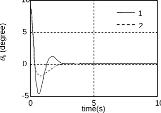
If we carry out the control only using feedback controller, we can see that the result is convergent. Nevertheless, if we use the same feedback controller and add a cerebellar cortex as a feedforward controller, we would get a better result. The simulation result is shown in Figure 7.
From Figure 7 we can see that the result with NNAC control is better than the feedback control result. The vibration amplitude is smaller.
5
0
-5 10
1 2
1 2
0.05
0 0.1 0.15
-0.05
0 1 2 3 4 5
time(s)
θb
(
de
gree
)
0 5
x(
m
)
Figure 7 Simulation results with On-line NNAC and feedback controller. The real line (1) denotes the control result with only the feedback controller, while the dashed line (2) denotes the result with on-line NNAC.
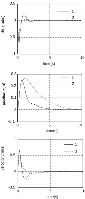
Now let’s detect its anti-interference performance. A step signal with amplitude 1 was given to the body of the robot. The experiment results are shown in Figure 8. We can find that the robot can generate a little angle to balance the step disturb and become stable at a certain point within a period of time.
0 5 10
-1 -0.5
0 0.5
time(s)
d
θb
(
rad/s)
15
time(s)
0 1 2 3 4 5
-1 -0.5 0 0.5
d
θb
(rad
/s)
1
2
0 5 10
-0.2 0 0.2
0.4 0.6
time(s)
velocity v(
m/s)
0 5 10
-0.2 0 0.2 0.4 0.6
time(s) 1
2
v(
m
/s)
15
Figure 8 Simulation results using On-line NNAC with a step disturb.
Figure 9 shows the different result between the On-line NNAC and traditional feedback control with step disturb.
0 5 10 15
-4 -2 0 2 4 6 8 10
time(s)
θb
(
degr
ee
)
feedback with FEL
τd
feedback only
Figure 9 Simulation results respectively using On-line NNAC. and feedback controller with a step disturb.
When the mass of robot body have some change. Through the simulation experiments, the mass M changes from 10kg to 30kg. Result analysis of comparative experiment can be made from Figure 10. In contrast to Figure 7, the traditional feedback control appears obvious vibrating when the mass of body became to 30kg, while there is not obvious change with On-line NNAC method (in Figure 10). These phenomenons illustrate that cerebellar cortex play an important part in the accurate balancing control and can effectively eliminate the shaking due to the system changing.
0 5 10 15
-5 0 5 10
time(s)
θb
(de
g
ree
)
0 5 10 15
0 0.1 0.2 0.3 0.4
time(s)
position x(m)
0 5 10
-5 0 5 10
time(s)
θb
(degr
ee)
Figure 10 Simulation results with feedforward controller and feedback controller when M was changed to 30kg.
TABLE II
CONTRASTIVE ANALYSIS
M Method Overshoot σ Response time t s On-line NNAC 14.82% 1.4754s 10kg
feedback 22.60% 1.9477s
On-line NNAC 20.38% 1.8883s 30kg
feedback 51.80% 2.2182s
From Table II, we can find that, no matter when mass is 10kg or 30kg, the overshoot and the response time with on-line NNAC method is little than with traditional feedback control. Especially, when the mass changes from 10kg to 30kg, the response all became slow to a certain extent. However, the overshoot with our proposed method changed from 14.82% to 20.38%, while the overshoot with traditional method had a larger change from 22.60% to 51.80%. From this point, we can conclude that, the on-line NNAC imitating the sensorimotor system and CNS can adap environment change and have an stable control effect.
CONCLUSION
V.
0 5 10
-1 -0.5 0 0.5 time(s) d θb (rad/s) 1 2
On the Neurophysiological concept, a biomimic control structure was designed based on the sensorimotor system and the central nervous system of human brain. The Research focused on the cerebellar cortex functioning in supervised training. An on-line NNAC method based on cerebellar model with feedback-error-learning on the neurophysiological mechanism was proposed to control the balancing two-wheeled robot which is a bionic self-balancing plant imitating human being. The cerebellar cortex as a forward controller was an on-line neural network adaptive controller and reflected the cerebellar function in balancing control problem. Through three representative simulation experiments including balancing control experiment, disturb experiment and mass changed experiment, we can see that the robot can be balanced in fixed position well by the biomimic control structure, and can get a better result comparing the traditional feedback control through the contrast of overshoot and response time.
time(s)
0 5 10
-0.1 0 0.1 0.2 0.3 position x(m) 1 2
APPENDIX A. PARAMETER UPDATE DEDUCING
2 2
1
2 2 2 2
2 2
2 2 2 2
(1) (1) (2) (2)
( ) (1, ) (1, ) (2, ) (2, )
(2) (2) (1) (1)
0; 0
(1, ) (1, ) (2, ) (2, )
ff ff
ff ff
u N u N
A j
W j W j W j W j
u N u N
W j W j W j W j
∂ ∂ ∂ ∂ = = = = ∂ ∂ ∂ ∂ ∂ ∂ ∂ ∂ = = = = ∂ ∂ ∂ ∂ time(s)
0 5 10
-0.5 0 0.5 1 velocity v( m/s) 1 2
(
)
(
)
(
)
(
)
(
)
(
)
T T 2 2 T T 1 T T 2 2 T T 1 (1) d (1, )0 (1 )
d (1, )
( ) 0 (1 )
(2) d (2, )
0 (
d (2, )
0 ( ) (1 )
( 1 6)
ff fb fb ff fb fb u W j u k
t W j
A j u k
u
W j
u k
t W j
A j u k
j η μ η μ μ η μ η μ μ ∂ ⎛ ⎞ = − ⎜ ⎟ + − ∂ ⎝ ⎠ = − + − ∂ ⎛ ⎞ = − ⎜ ⎟ + − ∂ ⎝ ⎠ = − + − = e e e e " 1 ) μ μ
(
)
(
)
(
)
(
)
T T 2 T T 2 d (1)1 0 (1 )
d d (2)
0 1 (1 )
d fb fb u k t u k t η μ μ η μ μ = − − + − = − − + − b e b e
(
T)
1 1 1 (1) (2) d (1 ) d ff ff fb u u W u k
t η W W μ
∂ ∂
⎛ ⎞
= − ⎜ ⎟ + −
∂ ∂
⎝ ⎠ μ e
1 1
1 1 1 1
(1) (1)
( , ) ( , )
ff ff
u u A N
W i j A N W i j
∂ ∂ ∂ ∂ = ∂ ∂ ∂ ∂ 6 2 1 1 2 1 1 6 2 1 2 1 ( ) (1 ( )) (1, )
( , )
(1 ( )) (1, ) ( )
j
j
N j
A j W j
W i j
A j W j e i
= = ∂ = − ∂ = −
∑
∑
In the same way,
(
)
6 2 1 2 1 1 T T 2 (1)(1 ( )) (2, ) ( ) ( , ) (1 ) ff j fb u
A j W j e i W i j
D W μu μ k
6 2 1
1 1 d ( , )
(1 ( )) ( ) ( )
d j
W i j
A j e i D j
t η =
= −
∑
−(
T)
1
1 1
(1) (2)
d
(1 )
d
ff ff
fb
u u
u k
t η μ
∂ ∂
⎛ ⎞
= − ⎜ ⎟ + −
∂ ∂
⎝ ⎠
b
e
b b μ
6 2
1 1
1 2
1
1 1 1 1
(1) (1)
(1 ( )) (1, )
( ) ( )
ff ff
j
u u A N
A j W j
j A N j =
∂ ∂ ∂ ∂
= = − −
∂b ∂ ∂ ∂b
∑
In the same way,
(
)
6 2
1 2
1 1
T T
2 (1)
(1 ( )) (2, )
( , )
(1 )
ff
j fb
u
A j W j
W i j
D W μu μ k
=
∂
= − −
∂
= + −
∑
e So that
6 2 1
1 1 d ( )
(1 ( )) ( )
d j
j
A j D j
t η =
=
∑
−b
(
)
(
)
T T
2
1
T 2
6 2 1
1 1 6
2 1
1 1
d
(1 ) d
d
(1 ) d
d ( , ) (1 ( )) ( ) ( ) d
d ( )
(1 ( )) ( ) d
( 1 6; 1 6)
fb fb
j
j
W
u k A
t
u k
t
W i j A j e i D j t
j
A j D j t
i j
η μ μ
η μ μ
η
η
=
=
⎧ = − + −
⎪ ⎪
⎪ = + −
⎪⎪ ⎨
⎪ = − −
⎪ ⎪
⎪ = −
⎪⎩
= =
∑
∑
e
b
e
b
" "
(5)
ACKNOWLEDGMENT
The authors gratefully acknowledge the national 863 plan projects (2007AA04Z226), NSFC(60774077), Beijing educational committee emphasis project
(KZ200810005002), Natural Science Fund of
Beijing(4102011) for the financing of the working and the assistance of teachers and classmates.
REFERENCES
[1] K Pathak, J Franch, S K Agrawal. Velocity and Position Control of a Wheeled Inverted Pendulum by Partial Feedback Linearization [J]. IEEE Trans. on Robotics (1552-3098), 2005, 21(3): 505-513.
[2] A Blankespoor, R Roemer. Experimental verification of the dynamic model for a quarter size self-balancing wheelchair. [C]// Proc. ACC. Boston: ACC, 2004: 488-492. [3] F Grasser, A D’Arrigo, S Colombi, A Rufer. Joe: A mobile, inverted pendulum [J]. IEEE Transactions on Industrial Electronics (S0278-0046), 2002, 9(1):107-114.
[4] NBot Balancing Robot, a two wheel balancing robot.
(2003). [Online].
Available:http://www.geology.smu.edu/~dpa-ww/robo/nbot/index.html.
[5] DING Xue-ming; ZHANG Pei-ren; YANG Xing-ming; XU Yong-ming. Motion Control of Two-wheel Mobile Inverted Pendulum Based on SIRMs [J]. Journal of System Simulation (in Chinese).2004,16(11):2618-2621.
[6] CHEN Xing; WEI Heng-hua; ZHANG Yu-bin. Modeling of Dual-wheel Cart-Inverted Pendulum and Robust Variance Control[J]. Computer Simulation(in Chinese). 2006,23(3) : 263-266.
[7] Chih-Hui Chiu. The Design and Implementation of a Wheeled Inverted Pendulum Using an Adaptive Output
Recurrent Cerebellar Model Articulation Controller [J].IEEE Transactions on Industrial Electronics. 2010, 57(5):1814-1822.
[8] Y. S. Ha and S. Yuta, “Trajectory tracking control for navigation of the inverse pendulum type self-contained mobile robot,” Robot. Autonom. Syst., vol. 17, no. 1/2, pp. 65–80, Apr. 1996.
[9] S. Jung and S. S. Kim, Control experiment of a wheel-driven mobile inverted pendulum using neural network. IEEE Transactions on Control Systems Technology. 2008, 16(2): 297–303.
[10]Kawato, M., Furawaka, K., Suzuki, R. A hierarchical neural network model for the control and learning of voluntary movements. Biol Cybern, 1987,56, pp. 1-17. [11]Kawato, M. Feedback-error-learning neural network for
supervised motor learning. In Advanced neural computers (ed. R. Eckmiller) 1990, pp. 365–372.
[12]M. Kawato, H. Gomi, A computational model of four regions of the cerebellum based on feedback error learning. Biol. Cybern. 69 (1992)95–103.
[13]Jun Nakanishi, Stefan Schaal. Feedback error learning and nonlinear adaptive control. Neural Networks. 2004,17:1453-1465.
[14]James C.Houk and Steven P.Wise. Distributed modular architectures linking basal ganglia, cerebellum, and cerebral cortex: their role in planning and controlling action. Cereb.Cortex. 1995,5:95–110.
[15]Doya, K. What are the computations of the cerebellum, the basal ganglia and the cerebral cortex? Neural Networks. 1999, 12: 961–974. (doi:10.1016/S0893-6080(99)00046-5) [16]J.C Houk, C Bastianen,etc. Action selection and
refinement in subcortical loops through basal ganglia and cerebellum. Phil. Trans. R. Soc. B. 2007,362:1573-1583(doi: 10.1098/rstb.2007.2063).
[17]Houk, J. C. Agents of the mind. Biol. Cybern. 2005,92:427–437. (doi:10.1007/s00422-005-0569-8) [18]Ito, M. Neurophysiological aspects of the cerebellar motor
control system[J] International journal of neurology, 1970.7 (2), pp. 162-176.
[19]Ruan, Xiaogang ; Ding, Mingxiao; Gong, Daoxiong; Qiao, Junfei On-line adaptive control for inverted pendulum balancing based on feedback-error-learning[J]. Neurocomputing, v 70, n 4-6, January, 2007, p 770-776.
Xiaogang Ruan, born in Sichuan Province, China in 1958, and received Ph.D. degree from Zhejiang University in 1992, Hangzhou, China. Now he is a professor of the Beijing University of Technology, and he is also as a director of IAIR(Institute of Artificial Intelligent and Robotics). His research interests include Automatic Control, Artificial Intelligence, and Intelligent Robot.