Adaptive Control based Particle Swarm
Optimization and Chebyshev Neural Network for
Chaotic Systems
Zhen Hong*
Faculty of Mechanical Engineering & Automation, Zhejiang Sci-Tech University, Hangzhou, China Email: [email protected]
Xile Li
Faculty of Mechanical Engineering & Automation, Zhejiang Sci-Tech University, Hangzhou, China Email: [email protected]
Bo Chen
College of Information Engineering, Zhejiang University of Technology, Hangzhou, China Email: [email protected]
Abstract—The control approach for chaotic systems is one of the hottest research topics in nonlinear area. This paper is concerned with the controller design problem for chaotic systems. The particle swarm optimization (PSO) algorithm is firstly proposed to search for the weights of the Chebyshev neural networks (CNNs), and then an adaptive controller for the chaotic systems is designed based on the PSO and CNNs. Moreover, it is proved that the designed controller can guarantee the stability of chaotic systems. Numeral simulation shows the effectiveness of the proposed method in the Logistic chaotic system.
Index Terms—adaptive control, particle swarm optimization, Chebyshev neural networks, chaotic systems
I. INTRODUCTION
Since the control approach for the chaotic systems was firstly proposed in [1], controlling chaotic system has become a hot research topic in nonlinear areas. Therefore, there are many approaches solving the control problem of chaotic systems, such as feedback control of chaotic system, adaptive control of chaotic system, state feedback law [2-4]. These methods are required to control all states of the system. However, in the actual engineering system, some state variables cannot be controlled directly. To overcome these drawbacks, it is interesting and important for finding the suitable practical control method in engineering application.
The neural network can learn and approach any nonlinear and uncertain system dynamics model with arbitrary precision, thus it provides new ideas and methods to solve the control problem for chaotic systems.
In this case, the chaotic control methods designed by using neural networks have made some achievements [5-12]. On the other hand, the studies in [13] show that the neural network with the orthogonal polynomial function has global approximation properties for approaching continuous function on any compact set with arbitrary precision. Particularly, when the orthogonal polynomial function is taken as Chebyshev polynomial, the performance of the designed neural networks is optimal. The reason is that the connection weights of Chebyshev neural networks (CNNs) is determined by the unidirectional gradient method, which is easy to make the objective function into local optimal impacting the efficiency of such neural network. Additionally, the particle swarm optimization (POS) adopts the speed-displacement search model, where the computational complexity is low, and the optimal solution is obtained by the cooperation and competition between particles. In this sense, the weights of the neural networks (NNs) are trained by using POS, which can give full play to the global optimization capability and rapid local convergence advantages for the PSO. Moreover, the PSO algorithm can also improve the generalization and learning capability of neural network [14]. These advantages of the PSO algorithm and CNNs motivate us to develop a control approach based on the PSO and CNNs for chaotic systems. Furthermore, to be best of the author’s knowledge, few results have been reported on this issue.
Motivated by the aforementioned analysis, the PSO algorithm is utilized to determine the connection weights of the CNNs, thus a novel CNN algorithm based on the PSO is proposed. In this case, we use the proposed algorithm to design an adaptive controller for the chaotic system. Since the convergence interval of Chebyshev basis function is in [-1, 1], an S-type function is introduced to extend its input range
[
−∞ +∞
,
]
, whichManuscript received November 16, 2013; revised December 25, 2013; accepted January 5, 2014.
expends the scope of application of such neural network. It is proved that the model of neural networks has good approximation performance for the multivariate polynomial. Finally, the one-dimensional Logistic chaotic system is given to demonstrate the effectiveness of the proposed method.
II. CNNLEARNING ALGORITHM FROM PSO A. Improved CNNs
First, the Chebyshev orthogonal polynomials [15] can be expressed as:
( ) cos( arccos( )), | | 1
n
T x = n x x ≤ (1) where T0(x)=1, T1(x)=x, and the recurrence formula is:
) ( ) ( 2 )
( 1
1 x xT x T x
Tn+ = n − n−
(2)
Since the range of x is
[ 1,1]
−
, and this condition will restrict the applications of CNNs, we introduce the following S-type function:1 1
2 )
( −
+
= −
x
e x
g α (3)
where the domain of the Eq.(3) is
[
−∞ +∞
,
]
, but the range ofg x
( )
is[ 1,1]
−
. Meanwhile, the variableα
in the functiong x
( )
is a tunable parameter. Then substituting Eq.(3) into Eq.(1) yields:( ) ( ( )) cos(arccos ( ))
2
cos arccos 1
1
n n
x
C x T g x g x
n
e−α
= =
⎛ ⎛ ⎞⎞
= ⎜ ⎜ − ⎟⎟
+
⎝ ⎠
⎝ ⎠
(4)
where 0 1
2
( ) 1,
( )
1
1
xC x
C x
e
−α=
=
−
+
, and Cn(x) isorthogonal polynomial satisfying
) ( ) ( 1 1
2 2 )
( 1
1 C x C x
e x
Cn+ − x ⎟ n − n−
⎠ ⎞ ⎜
⎝
⎛ −
+
= α (5)
X
. . . 1
1
1
Incentive function (Input layer)
Y
W0
W1
Wm Chebyshev orthogonal
Hidden layer
0( )
C x
( )
m
C x
1( )
C x
Linear incentive Output layer
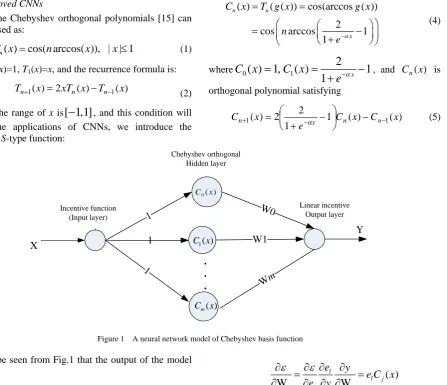
Figure 1 A neural network model of Chebyshev basis function
It can be seen from Fig.1 that the output of the model is:
0
W ( )
m j j j
y C x
=
=
∑
(6)where the improved Chebyshev function C xj( ) is determined by (5). It is assumed that the desired output is
y
d, then the error function is defined by el yd −y. Under this condition, the objective function of optimization problem is:(
)
22
1 1
1 1
2 2
r r l d l l
e y y
ε
= =
=
∑
=∑
− (7)where
r
denotes the number of training samples. It follows from the gradient descent method that the learning rule of Wj is:( )
W W
l
l j j l j
e y
e C x
e y
ε
ε
∂∂ = ∂ ∂ =
∂ ∂ ∂ ∂
As mentioned before, one has
W (j t+ =1) W ( )j t +
η
e C xl j( ) (8) whereη
is the learning rate, and0
< <
η
1
.improve the efficiency of neural network algorithm, and the convergence performance can be improved. In what follows, we firstly give the detailed mathematical description of the PSO:
Suppose that Ω ⊂Rn is a target search space of n-dimension, and a group X ={ ,x x1 2,",xn} is composed by n particles. Then the velocity and position of the ith particle is defined by:
T
1 2
T
1 2
( ) [ ( ) ( ) ( )] ,
( ) [ ( ) ( ) ( )]
i i i in i i i in
v k v k v k v t
x k x k x k x k
"
"
And the current individual optimal solution of the ith particle is:
1 2
pbest ( )i k (p ki ( ) pi ( )k " pin( ))k The current group optimal solution is:
1 2
gbest( ) ( ( ), ( ), , ( ))
n
g g g
k g k g k " g k
where k is the number of current evolution generation. According to the theory of optimal particle tracking, the particle
x
i updates its velocity and position according to the following formula:1 2
( 1) ( ) ( )
rand(0,1) (pbest ( ) ( ))
rand(0,1) (gbest ( ) ( )) ( 1, 2, , )
id id
i id
g id
v k w k v k
c k x k
c k x k i n
+ =
+ ⋅ ⋅ −
+ ⋅ ⋅ − = "
(9)
( 1) ( ) ( 1)
id id id
x k+ =x k +v k+ (10)
where the Eq.(9) and Eq.(10) describe the update mode of particles’ velocity and position, respectively. The parameters c1 and c2 are the accelerated constant, and their selected values are in [0, 2]. w k( )is a linear inertia weight index. If the value of w k( ) is relatively large, the global convergence will be better. Otherwise, the local convergence is better. w k( ) is taken as:
( ) 0.9 0.5
MaxNumber
k
w k = − ⋅
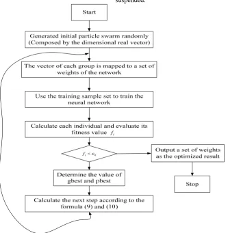
Where the "MaxNumber'' is the maximum iterations. For the neural network model in Section II(A), we make the connection weights Wj of CNNs as the position vector x in the PSO algorithm. We also determine the fitness function in particle swarm optimization according to the Eq.(7). Given a set of initial velocity randomly, and using the PSO algorithm to conduct iteration training, when the fitness function is less than the given error range, fi<
ε
0, the algorithm is suspended.i
f
0
i
f <ε
III THE CONTROLLER DESIGN BASED ON CNNS AND
PSO
Considering the following chaotic system:
) ), ( ( ) 1
(k f x k p
x + = (11)
where x∈Rn is the system status, and p is the system parameter.
Using the neural network learning algorithm based on the PSO to simulate the input-output relationship of chaotic model (11), one has
) ), ( ( ˆ ) 1 (
ˆ k f x k p
x + = (12)
According to the system stability theory, the controller can be taken as:
)) ( ) ( ( ) 1 ( ) ), ( ( ˆ )
(k f x k p x k x k x k
u =− + d + +β − d (13)
where
x
d is the desired target track,β
is theparameter. Then combining Eq.(12) and Eq.(13) yields:
ˆ
( 1) ( ( ), ) ( ( ), )
( 1) ( ( ) ( ))
d d
x k f x k p f x k p
x k β x k x k
+ = −
+ + + −
(14)
If the proposed neural network can approach the system (11), then the error system is described by
) ( )) ( ) ( ( ) 1
(k x k x k e k
e + =β − d =β (15)
where e(k+1)=x(k+1)−xd(k+1).
According to the system stability theory, we assume 1
|
|β < , which guarantees the error system (15) is asymptotically stable. It is easy to prove that when the system (11) is applied to control, it can track the controlled objective. So the approximation performance of the neural network is particularly important. In what follows, we will discuss the demands of the fuzzy Chebyshev basis function neural network to the chaotic system control accuracy.
Definition 1 Suppose
∀ ∈
X
R
n, xn∈[a,b], g(X) is an n-polynomial and ||g(X)|| is bounded or integral in the domain, and if g(X) satisfies the following inner product relationship: [ , ] 2 [ , ] ( ( ), ( )) ( ) ( ) ( ) 0, = ( ) ( ) , nl k a b l k
n
l a b
g X g X X g X g X dX
l k
X g X dX l k
ρ ρ = = ⎧⎪ ⎨ ≠ ⎪⎩
∫
∫
(16)Then gn(X) sequence is called multivariate orthogonal
polynomial, and the weights are
ρ
( )
X
.For the n-dimensional vector X =[x1,x2,",xn]T , n-arid functionf(X) and multiple integral symbols, we make the convention as:
,
[ , ]
i i
x
X x
a b
∀ ∈
∈
is recorded asx
n∈
[ , ]
a b
," 个 n b a b a b a
∫ ∫ ∫
is recorded as [ ]∫
n ba, , dx dxn
"
1 is
recorded as dX.
Considering the multivariate polynomial composed by orthogonal polynomial, one has
1
( ) ( )
n
i i
j
g X C X
=
=
∏
(17)On the other hand, Chebyshev orthogonal polynomial satisfies the following inner product relationship:
1 1 1 2 1 ( ( ), ( )) ( ) ( ) ( ) 0, = ( ) ( ) ,
l k l k
l
C x C x x T x T x dx
l k
x T x dx l k
ρ
ρ
− − = = ⎧⎪ ⎨ ≠ ⎪⎩∫
∫
(18)where
x
∈
R
.Substituting Eq.(17) into Eq.(18) yields:
[ 1,1] [ 1,1] 1 1 ( ( ), ( )) ( ) ( ) ( ) = ( ) ( ) ( ) n
l k l k
n n
n
l j k j
j j
g X g X X g X g X dX
X C x C x dX
ρ ρ − − = = =
∫
∏
∏
∫
(19)Since the orthogonal polynomial C0(x), C1(x), …, Cn(x)
is linearly independent, the integral order of the Eq.(19) can be changed, then:
[ 1,1] 2 [ 1,1] ( ( ), ( )) ( ) ( ) ( ) 0, = ( ) ( ) , n
l k l k
n
l
g X g X X g X g X dX
l k
X g X dX l k
ρ ρ − − = = ⎧⎪ ⎨ ≠ ⎪⎩
∫
∫
(20)Obviously, Eq.(20) satisfies the condition in Definition 1, which is a multivariate orthogonal polynomial, and
x
n∈ −
[ 1,1]
.Definition 2 For a given function f(X) which the
range is xn∈[−1,1] , using the polynomial
) ( ) ( 1 X g W X y n k k k
∑
== to make the optimization mean
square approximation and find out the value )
, 2 , 1
(i n
Wi = " to make the function
dX X y X f X X y X f n
∫
− − = − ] 1 , 1 [ 22 ( )[ ( ) ( )]
) ( )
( ρ is the
minimum.
Lemma 1[13] A neural network based on the orthogonal polynomial possesses the global approximation property for arbitrary precision approaching continuous function on any compact set.
Theorem 1 According to Eq.(11), utilizing the
based on the PSO, we can get the neural network model (12) for the chaotic system. Using the controller designed by Eq.(13) to chaotic system (11), then there exists a positive constant
σ σ
(
>
1)
such that| ) ( | | ) (
|e k <σ fe k , where
e k
( )
andf k
e( )
denotesthe tracking error and model error, respectively.
Proof: Let us denote 1 sup|e(k)|
k
=
γ
and 2 sup| fe(k)|
k
=
γ . If we want to prove
| ( ) |
e k
<
σ
|
f k
e( ) |
, we just need to proveγ
1≤
σγ
2. It follows from Eq.(14) that) ( ) ( ) 1
(k f k e k
e + = e +β .
Taking the absolute value on both sides of the equation above, one has:
| ) ( | | ) ( | | ) ( ) ( | | ) 1 (
|e k+ = fe k +βek ≤ fe k + βe k (21) Taking the maximum on both sides of the Eq.(21), one has
1 2
|
|
1γ
≤ +
γ
β γ
where |β|<1.
Consolidating the above equations yields
2 1
| | 1
1 γ
β γ
− ≤
Then we denote
| | 1
1
β σ
−
= , one has
2 1
σγ
γ
≤
where it is obvious that
σ
>
1,
which implies that| ( ) |
e k
<
σ
|
f k
e( ) | .
Remark: Theorem 1 denotes that the tracking error cannot be less than the model error. Therefore, the model error on the stability of the system is an extremely important role that the higher accuracy of the model, the higher accuracy of the control.
IV THE NUMERICAL SIMULATION
We use the Logistic chaotic system to check the effectiveness of the chaos control method. The details are as follows.
Logistic mapping system is:
)) ( 1 )( ( ) 1
(k x k x k
x + =λ − (22)
where x∈[0,1] and
λ
is a positive constant. When4
=
λ
, the system is in a chaotic state.Supposing
η
=
0.05
,α
=
0.01
, and using the fuzzy Chebyshev neural network learning algorithm (22), we can get a model as follows:)) ( ( ˆ ) 1 (
ˆ k f x k
x + =
According to the Eq.(13), a desired controller is as follows:
)) ( ) ( ( ) 1 ( )) ( ( ˆ )
(k f x k x k x k x k
u =− + d + +β − d
Figure 3
Figure 4
When the control is exerted, the system (22) is changed as:
) ( )) ( 1 )( ( ) 1
(k x k x k u k
x + =λ − + (23)
Whenλ=4,β=0.02, the designed control targets are 7
. 0 ) (k =
xr andxr(k)=0.5+0.2sin(kπ/100).
When the control is exerted at the 100th step, the control results are showed in figure 3 and figure 4, respectively.
V CONCLUSION
An adaptive control method based PSO and CNNs is proposed for chaotic systems. The PSO algorithm is mainly used to search for the weights of the CNNs. Then, an adaptive controller for the chaotic systems is designed using the approach which is combined with PSO and CNNs. Furthermore, we prove that the designed controller can guarantee the stability of chaotic systems.
The number of iterations i
The o
u
tp
ut
val
u
e X(
k)
The control objective X r=0.7
The number of iterations i
The o
u
tp
ut
val
u
e X(
k)
Finally, the Logistic chaotic system is given to demonstrate the effectiveness of the proposed method.
ACKNOWLEDGMENT
This work was supported by National Natural Science Foundation of China (61304256), Zhejiang Provincial Natural Science Foundation of China (LQ13F030013), project of Education Department of Zhejiang Province (Y20132700), Ningbo Natural Science Foundation (2012A610016) and Science Foundation of Zhejiang Sci-Tech University (1202815-Y).
REFERENCES
[1] E. Ott, C. Grebogi, and J. A. Yorke, “Chaos control,”
Physical Review Letters, vol. 64, no. 11, pp. 1196-1199, 1990.
[2] G. Chen, “Controlling chaos and bifuractions in
engineering systems”, CRC press, 2000.
[3] W. Sanum, and B. Srisuchinwong, “Highly complex
chaotic system with piecewise linear nonlinearity and
compound structures,” Journal of Computers, vol. 7, no. 4,
pp. 1041-1047, 2012.
[4] X J Li, W X Xiao, Z Liu, W L Wan, and T S Hu, “A new
fractional order chaotic system and its compound
structure," Journal of Software, vol. 8, no. 1, pp. 126-133,
2013.
[5] P. M. Alsing, A. Gavrielides, “Using neural networks for
controlling chaos,” Physical Review E, vol. 49, pp.
1225-1231, 1994.
[6] C. T Lin, “Controlling chaos by GA-based reinforcement
learning neural networks,” IEEE Transactions on Neural
Networks, vol. 10, no. 4, pp. 846-859, 1999.
[7] C. F Hsu, “Intelligent control of chaotic systems via
self-organizing Hermite-polynomial-based neural
network,” Neurocomputing, vol. 123, pp. 197-206, 2014.
[8] P. Yadmellat, S. K. Y. Nikravesh, “A recursive delayed
output-feedback control to stabilize chaotic systems using
linear-in-parameter neural networks,” Communications in
Nonlinear Science and Numerical Simulation, vol. 16, no. 1, pp. 383-394, 2011.
[9] S. C. Jeong, D. H. Ji, J. H. Park, S. C. Won, “Adaptive
synchronization for uncertain chaotic neural networks with mixed time delays using fuzzy disturbance observer,”
Applied Mathematics and Computation, vol. 219, no. 11, pp. 5984-5995, 2013.
[10]L S Yin, Y G He, X P Dong, and Z Q Lu. “Multi-step
prediction algorithm of traffic flow chaotic time series
based on volterra neural network," Journal of Computers,
vol. 8, no. 6, pp. 1480-1487, 2013.
[11]W Tan, Y N Wang, Z R Liu,and S W Zhou, “Controlling
chaotic system by RBF neural networks nonlinear
compensator,” Control Theory & Applications, vol. 20, no.
6, 951-954, 2003. (In Chinese)
[12]D Liu, H P Ren, and Z Q Kong, “Control of chaos solely
based on RBF neural network without an analytical
model,” Acta Physica Sinica, vol. 52, no. 3, pp. 533-535,
2003. (In Chinese)
[13]X J Wu, S T Wang, J Y Yang, and Q Y Cao, “The study on
the orthogonal polynomials-based neural networks and its
properties,” Computer Engineering and Application, vol.
39, no. 9, 25-27, 2002. (In Chinese)
[14]J. R Zhang, J Zhang, T. M Lock, and M. R. Lyu, “A hybrid
particle swarm optimization—back-propagation algorithm
for feedforward neural network training,” Applied
Mathematics and Computation, vol. 185, pp. 1026-1037, 2007.
[15]V Basios, A. Yu. Bonushkina, and V. V. Ivanov, “On a
method for approximatin one-dimensiona functions,”
Computer and Mathematics with Applications, vol. 34, pp. 687-693, 1997.
Zhen Hong received both B.S. degrees from Computer Science & Technology at Zhejiang University of Technology, Hangzhou, China and Computing at University of Tasmania, Australia, respectively. He received Ph. D. degree in Control Theory and Control Engineering at the College of Information Engineering, Zhejiang University of Technology, Hangzhou, China, in 2012. He is currently working as a lecturer at Faculty of Mechanical Engineering & Automation, Zhejiang Sci-Tech University, Hangzhou, China.
His main research interests include wireless sensor networks, optimization, adaptive control and intelligent transportation.
Xile Li received the B.S. degree in Measurement Technology and Instrument at Faculty of Mechanical Engineering & Automation, Zhejiang Sci-Tech University, Hangzhou, China, in 2012. She is currently a Master student in Faculty of Mechanical Engineering & Automation, Zhejiang Sci-Tech University, Hangzhou, China.
Her main research interests include wireless sensor networks, topology control.
Bo Chen received the B.S. degree in Information and Computing Science from Jiangxi University of Science and Technology, Ganzhou, China, in 2008. He is currently working toward the Ph.D. degree in Control Theory and Control Engineering at the College of Information Engineering, Zhejiang University of Technology, Hangzhou, China.