A Systematic Approach to Adaptive Dimensioning of Data Centers

A Systematic Approach to Adaptive

Dimensioning of Data Centers

Wenhong Tian

a _{School of Computer Science and Engineering}

University of Electronic Science and Technology of China Chengdu 611731, China

Email: tian [email protected]

Abstract— Cloud data centers (CDCs) provide key infras-tructure for Cloud computing. Accurately allocating com-puting resources is very important for the CDCs to function efficiently. Current allocation of resources in CDCs is mostly dedicated and static. However, workloads for Cloud appli-cations are highly variable which cause poor application performance, poor resource utilization or both. In this paper, considering both blocking and delay probability by applying queuing theories to model different scenarios, systematic adaptive dimensioning methods for CDCs are developed so that right amount of computing resources are allocated for variable workloads to meet quality of service requirements in different situations. Both single CDC and multiple CDCs with and without delay are considered. The proposed methods can be applied to dimension data centers efficiently and dynamically.

Keywords: Cloud computing; Cloud Data Centers (CDCs); Adaptive Dimensioning Methods.

I. INTRODUCTION

Cloud Computing refers to the applications delivered as services over the Internet, the hardware and sys-tems software in the data centers that provide those services [1] [3]. Cloud data centers (CDCs) consist of both clustering of servers and networking infrastructure. Driven by the economics of large number of low-cost servers with clustering, the reliability and availability of the Cloud system as a whole are improved significantly in distributed computing. Current CDCs, for instance, Google’s, Amazon.com’s, and Microsoft’s, now being built to contain more than 100,000 servers. Google [2] introduces one of CDC architecture: which consists of multiple clusters distributed worldwide. Each cluster has around a few thousand machines, and the geographically distributed setup protects the system against catastrophic data center failures (like those arising from earthquakes and large-scale power failures). The servers on each side of a rack interconnect via a 100-Mbps Ethernet switch that has one or two gigabit uplinks to a core gigabit switch which connects all racks together. In Amazon.com [7], the virtual machine providing the equivalent of a system with a 1.7Ghz x86 processor, 1.75GB of RAM, 160GB of local disk, and 250Mb/s of network bandwidth,

Manuscript received Feb. 12, 2013; revised June 14, 2013; accepted July 4, 2013. c2005 IEEE.

This work is supported the National Natural Science Foundation of China (NSFC) Grant 61150110486.

(4280 hosts), and Eastern Asia (2396 hosts). New hosts added per day and average new hosts per day are shown in Figure 2 and Figure 3 respectively. It can be seen that customer requests (hosts) are highly variable. We need to develop adaptive dimensioning methods so that right amount of computing resources can be allocated for variable workload to avoid overprovisioning or under-provisioning. An architecture and server migration

Figure 1. An Example of Requests Arrival Rate from [19]

Figure 2. New Hosts For SETI@home [30]

Figure 3. Average New Hosts For SETI@home [30]

approaches have been introduced in [19] where both online and offline server migration strategies are discussed and evaluated. Liu et al. [18] propose an architecture of self-adaptive configuration optimization system which supports dynamic reconfiguration when workloads change using genetic algorithm. An integer linear programming

BR: border router

AR: access router

LB: load balancer

A: rack of servers

DIP:direct IP address

VIP:virtual IP address

Figure 4. A New Architecture for Data Center [10]

(ILP) approach is provided in [6] to solve the resilient grid/cloud dimensioning problem using failure-dependent backup routes. Next generation architecture for data cen-ters is proposed in [10] and reprinted in Figure 4. In the architecture, layer 2 networks connect all the servers inside a data center and requests are distributed over pools of servers. To increase the total capacity of the CDCs, three layered structure of internetworking is proposed in [10] and reprinted in Figure 5. There are n1 = 144

Figure 5. Three layered structure for Data Center [10]

CDC architectures are manually configured and cannot automatically adapt to time-varying workloads, they re-sult in poor resource utilization when workload is low (overprovisioning) or significant performance degradation when loads exceed capacity (under-provisioning) as dis-cussed in [19]. To overcome overprovisioning and under-provisioning problems, adaptive dimensioning methods are developed in this paper. The paper is organized as follows. In section II, methods for adaptive dimensioning of single Cloud data center are proposed. Method for multiple federated Cloud data centers is discussed in section III. Finally, the conclusions are given in section IV.

II. SINGLECLOUDDATACENTER(CLOUD)

In this section, models and dimensioning methods for single Cloud data center are discussed on the basis of blocking and non-blocking models.

A. Dimensioning with Blocking Models

Assuming that individual requests constituting the workload are independent to each other; tasks are sched-uled in a first-in-first-out manner without preemption; but the incoming requests that find all servers busy are blocked and depart from the system. Erlang loss model can be applied in this case.

1) Erlang Loss Model with Poisson Arrivals for Single Class of Customers (requests): In this case, a CDC with server cluster can be modeled as a M/G/C/C queue, i.e., requests arrivals follow Poisson process and service time distribution can be general and there are total C servers in a CDC. Provisioning optimal total number of servers is one of practical ways to meet the blocking probability and other QoS requirements. In this section, we describe how to calculate the minimum number of serversCof the blocking model so that the maximum blocking probability is less than a pre-specified valuefor a given load. Erlang loss formula is given by:

B(N, ρ) = ρ N_/N! PN

i=0ρi/i!

(1)

where ρ is the offered load to the system, for example measured by the number of requests per seconds. This minimum value of C can be calculated iteratively using equation (1). However, when the required capacity C is very large, this iterative approach becomes CPU intensive since its time complexity isO(log2(N/)N). A recursive formula for equation (1) is as follow:

B(N, ρ) = ρB(N−1, ρ)

N+ 1 +ρB(N−1, ρ), B(0, ρ) = 1. (2) It is a long-standing conjecture that the optimal number of servers is of the form ρ+K√ρfor Erlang loss model whereK is a constant depending on the offered load and blocking probability. This approximation yields very ac-curate results. Indeed, based on extensive sensitivity tests, the actual optimum and approximate values rarely deviate by more than one server, or by more than one percent,

TABLE I.

THE REQUIRED NUMBER OF SERVERSCVS.OFFERED LOAD(ρ)

ρ Method C ρ Method C

0.14 Exa 2 100 Exa 118

0.14 Asm 2 100 Asm 118

1 Exa 5 200 Exa 222

1 Asm 5 200 Asm 222

3 Exa 8 500 Exa 527

3 Asm 8 500 Asm 527

10 Exa 18 1000 Exa 1030

10 Asm 18 1000 Asm 1030

40 Exa 53 2000 Exa 2030

40 Asm 53 2000 Asm 2030

whichever is greater. In this paper, single class traffic is considered for a CDC. Then asymptotic expression for the optimum value of C is obtained as follow:

N =ρ+ψ(√ρ)√ρ (3) where is the blocking probability requirement, ρis the offered load (workload) to the system and ψ(x) is the unique solution of the following differential equation

ψ0(x) = −1

(ψ(x) +x)x), ψ( p

2/π) = 0 (4) In [22], equation (4) is solved to obtain

x−1e−0.5ψ(x)2−√2πerf(0.51/2ψ(x))−x√0.5π= 0 (5) whereerf(.)function is defined as follow:

erf(x) =√2

π

Z x

0

exp(−t2)dt (6) Given x, equation (4) can be easily solved numerically for ψ(x). Applied to equation (3), the requested total number of servers can be obtained.Table I shows the minimum required number of servers for a Erlang loss queue, so that the blocking probabilityis less than 0.01. The offered load ρwas varied. For each value of ρ, the minimum required servers is computed using equation (3) (labelled as ‘Asm’) and also using Erlang loss formula (exact solution labeled as ‘Exa’) which can be obtained using equation (2) iteratively. Through many numerical examples, that the minimum capacity C obtained using equation (3) is observed to be very closed to the exact solution.

2) Erlang Loss Model with Poisson Arrivals for Multi-ple Classes of Customers: Let us assume that the system has a total C identical servers, and each can provide service to any class of arrivals. Let n=(n1, n2, ..., nR) wherenris the number of classrcustomers in the system, and letb=(b1, b2, ..., bR). The total number of busy servers in state C is

bnT =b1n1+b2n2+...+bRnR. (7) The set of all possible states of the system can be described as

It is well known that the multi-class Erlang loss system has a product-form solution.

P(n) = R Y

i=1

ρni i

ni!

G−1(Ω),∀n∈Ω (9) where

G(Ω) =X n∈Ω

R Y

i=1

ρni_i ni!

(10)

The class-i has offered loadρi=λi/µi. The challenge in this model is to obtain the blocking probability for each class. Computing the blocking probabilities by directly enumerating all possible states of the system requires an O(CR) amount of time. The direct method is com-putationally cumbersome and grows exponentially fast even for relatively small systems. Several methods have been presented in the literature to avoid the exponential complexity of the computations. One of the most powerful methods for obtaining the blocking probabilities was pub-lished independently by Kaufman (1981) [14] and Roberts (1981) [20]. The Kaufman-Roberts method is a recursive algorithm that has a linear complexity, O(CR), and it is considered as a fast method. The recursive formula is as follows:

w(K) = 1

K

R X

r=1

ρrbrw(K−br), K= 1,2, ..., C. (11) wherew(x)=0 if x <0,w(0)=1 and ρr=λr/µr. Then, the blocking probability of classr arrivals is given by:

BPr= PC

j=C−(br−1)w(j) PC

j=0w(j)

, r= 1,2, ..., R. (12) It is interesting to know that this formula can be applied to the single class model, as a fast way of obtaining the blocking probability. Given the blocking probabilities, the average number of classr customers in the system is

E[Qr] =ρr(1−BPr), r= 1,2, ..., R. (13) 3) Blocking Model with General Arrival Processes for Single Class of Customers: Mt/G/N/N queue model can be applied for general arrivals which may be time varying. A solution similar to Erlang loss model is pro-vided in [11]:

N =bρt+ψ(

b

p

b2_ρ t)

p

b2_ρ

t (14)

where time-varying ρt is the offered load to the sys-tem and b is the bandwidth (servers) required by each request. A few examples are also introduced in [11]. Let us take one example from [11], arrival rate

λ(t)=40+10sin(2πt/80), requesting b=5 units of band-width (similar to servers in CDCs) and desiring no more than 1 percent blocking. Taking every 10 minutes as a measurement and provisioning interval. Figure 6 shows the dimensioning results for eight periods of measure-ment. Decisions of adaptive provisioning are made at the end of each measurement interval to meet the blocking probability of requirement.

Figure 6. Eight Periods Provisioning Example from [11]

4) Blocking Model with General Arrival Processes for Multiple Classes of Customers: Similar to Poisson arrival processes for multiple classes of customers, the total number of servers in general arrival case can be dimensioned using following equation:

C= R X

i=1

biρi(t)+ψ( min 1≤i≤R

i

bi v u u t

R X

i=1

biρi(t)) v u u t

R X

i=1

biρi(t) (15) where time-varying ρi(t) is the offered load to class-i,

i andbi is respectively the blocking probability and the number of servers requests for class-i.

B. Dimensioning with Nonblocking Models

Assuming that individual requests constituting the workload are independent to each other; tasks are sched-uled in a first-in-first-out manner without preemption; there are a large number of servers so that requests rarely incur blocking or non-blocking. Then delay models can be applied in this case.

1) Erlang Delay Model: Erlang delay modelM/M/C

λis the arrival rate and τ is the average service time:

D(C, A) =

AC C!(1−A) PC−1

k=0 Ak

k! + AC C!(1−A)

(16)

where A=ρ/C if ρ≤ C; A=1 if ρ=1. And for large C, computing D(C, A) directly is very expensive or can cause computer overflow. Notice that there is a recursive formula for Erlang B and a recursive formula based on Erlang B (equation (2)) can be used for Erlang C as follows:

D(C, A) = B(C, A)

1−A(1−B(C, A)) (17) It is obvious that the larger C is, the smaller delay will be. However, we cannot design the CDC to have as many servers as possible because of finance and space limitation. We can compute a few examples and find that D(0.9, 1)=0.9, D(9, 10)=0.67, D(90, 100)=0.22 and D(900, 1000)=0.0006. In all above cases, the server utilization is 0.9. It shows that large systems are more efficient than small ones. The following equation can be used to predict how long the customers (requests) will have to wait:

w=D(C, A) 1 1−A

τ

C (18)

This holds true even when service is not first come first service (FIFO), for example, LIFO (Last in First out) or service in random order. This is because that interchang-ing statistically identical customers waitinterchang-ing in the queue does not change the number of customers or the amount of work waiting to be served, see Cooper [5] for more detailed explanations. Tian and Perros [23] introduced one way to dimension the data center with job priorities and QoS constraints using single server queuing model. Based on Erlang delay model itself, it is possible to dimension the system to meet QoS requirements. Jennings et al [13] introduced the following formula for dimensioning Erlang delay model:

C=ρ+zα

√

ρ (19) where ρ is the mean offered load to the system. After some computation and simplification, zα satisfies

P r(N(0,1)> zα) =α= 1

√

2π

Z ∞

zα

exp(−u2/2)du

(20) whereN(0,1) is the standard normal distribution andα

is the delay probability of the system. Given α, zα can be computed explicitly so that the required number of servers C can be found easily from equation (19). It is shown in [13] that using equation (19) for dimensioning of Erlang delay model can meet given delay requirement with appropriate number of servers. Equation (19) and (20) can be easily used to find the appropriate number of servers. In Table II, the probability of delay as a function of the offered load in the Erlang delay queue M/M/C is shown, where C is chosen to satisfy Equation (20) with

α=0.005 (zα=2.576).C(Asm)is obtained using equation (19) while C(Ite) is obtained applying equation (16) iteratively.

TABLE II.

THE REQUIRED NUMBER OF SERVERSCVS.OFFERED LOAD(ρ) ρ ρ+zα

√

ρ C(Asm) C(Ite)

1 4.1 5 5

10 18.6 20 21

100 126.3 127 128

200 236.9 237 239

500 558.1 559 560

1000 1082.1 1083 1084 2000 2115.7 2116 2119

2) Nonblocking model with General Arrivals and Ser-vices: In this case, requests arrival process and service process can be general.

(1) Considering delay probability. In this case the total number of servers can be found using the following equation:

C=ρt+zα

√

ρt (21) where ρt is the mean time-varying offered load to the system.

(2) Considering response time. A CDC with server cluster can be modelled as a G/C/C system which has a mean response time R under heavy traffic given by [16]

R= 1 ¯

µ+ σ2

a+ σ_b2 C2

2t(1−U) (22) where σ2

a and σ2b are the variance of inter-arrival and service times, respectively, andtis the mean inter-arrival time, µ¯ is the mean service rate and U is the average CPU utilization in the previous measurement interval. U

can be obtained by taking average over all servers’ CPU utilization. It can be seen that the number of servers C

is related to six variables (R,U,µ¯,t,σ2

a,σb2). Solving the equation for C, we have

C= s

σ2 b 2t(1−U)(R−1

¯ µ))−σ

2 a

(23)

Given (R, U, µ¯, t, σ2

a, σb2), the required number of servers for the next interval can be computed using above equation. Normally, the quality of service (QoS) requirements may includeUandR. Andµ¯,t,σa2,σb2can be measured. For example, given U=0.5,t=0.2,σ2a=0.2 and

σ2

b=100, the total number of required servers is changing with the required response time R, results are shown in Figure 7.

C. Optimized Capacity Provisioning and Bounds

For the given arrival rate and blocking probability requirement of each class, we may use an iterative approach (based on fixed point algorithm) to optimize the total capacity. We are to find the number of total servers required for a CDC to meet the acceptable level of blocking (known as grade-of-service). The optimization problem is to find a minimum total number C for given offered load and acceptable blocking

Figure 7. A Dimensioning Example for Non-blocking Model

When needed capacity is very large, iterative approach based on fixed point algorithm will be expensive with time complexity at least O(CR). It is a long-standing conjecture the optimal number of bandwidth (servers) is of form servers=ρ+K√ρfor single class traffic whereK

is a constant depending on the offered load and blocking probability. In Grassmann [8], he stated that “Extensive sensitivity testing revealed that this approximation yields very accurate results. Indeed, the actual optimum and the approximation rarely deviate by more than one server, or by more than one percent, whichever is greater.” For multiclass traffic, similar result was introduced by Hampshire et al. in [10]:

C= R X

i=1

biρi+ψ( min 1≤i≤R

i

bi v u u t

R X

i=1

biρi) v u u t

R X

i=1

biρi (25) where i is the grade of service (blocking probability) requirement for class-i traffic and ψ(x) is the unique solution to the equation (5). Given x, equation (5) can be solved easily with complexity O(1), i.e., we can get

ψ(x)easily givenx. Applied to equation (25), we obtain the request total capacity. Because of the asymptotic rule, satisfying the requirements provides more than enough servers for all the other classes. Through many numerical examples, we observed that the total servers obtained using equation (25) is very closed to exact solution. This approach is a very accurate provisioning solution with complexityO(1). Also from Ross [20], we know that the blocking probability of each class is proportional to its servers (bandwidth) requirement when total capacity is very large, i.e.,

BPk≈bkα, k= 1,2, . . . , R (26) whereαis a constant for given total capacity and offered loads. If we know Qos requirement of the dominant Qos classes, we can know the blocking probabilities of other classes, so we can find total arrival rates for each class easily and then use equation(25) for provisioning. Observ-ing that the asymptotic rule of thumb and the blockObserv-ing probabilities relationship among different classes, we can

TABLE III.

8TYPES OF VIRTUAL MACHINES(VMS)INAMAZONEC2

MEM CPU (units) Sto VM

1.7 1 (1 cores×1 units) 160 1-1(1) 7.5 4 (2 cores×2 units) 850 1-2(2) 15.0 8 (4 cores×2 units) 1690 1-3(3) 17.1 6.5 (2 cores×3.25 units) 420 2-1(4) 34.2 13 (4 cores×3.25 units) 850 2-2(5) 68.4 26 (8 cores×3.25 units) 1690 2-3(6) 1.7 5 (2 cores×2.5 units) 350 3-1(7) 7.0 20 (8 cores×2.5 units) 1690 3-2(8)

TABLE IV.

3TYPES OF PHYSICAL MACHINES(PMS)SUGGESTED

PM CPU (units) MEM Type

1 16 (4 cores×4 units) 160 1 2 52 (16 cores×3.25 units) 850 2 3 40 (16 cores×2.5 units) 1690 3

find the blocking probability of the dominant Qos classes by inverting the equation (25) as follows:

i=

bi

δR∞ 0 e−0.5t

2_+(C−m)t/δ

dt (27)

where m (called mean of offered load) and δ (called standard deviation of offered load) are defined as:

m= R X

i=1

biρi;δ= v u u t

R X

i=1

b2

iρi (28)

Equation (27) and (28) can help us find the tight bounds of blocking probabilities given other parameters.

III. MODELINGVIRTUALMACHINESALLOCATION

TABLE V.

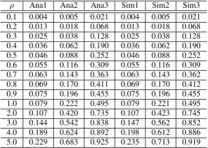
THE BLOCKING PROBABILITY COMPARISON FORPMTYPE1

ρ Ana1 Ana2 Ana3 Sim1 Sim2 Sim3

0.1 0.004 0.005 0.021 0.004 0.005 0.021 0.2 0.013 0.018 0.068 0.013 0.018 0.068 0.3 0.025 0.038 0.128 0.025 0.038 0.128 0.4 0.036 0.062 0.190 0.036 0.062 0.190 0.5 0.046 0.088 0.252 0.046 0.088 0.252 0.6 0.055 0.116 0.309 0.055 0.116 0.309 0.7 0.063 0.143 0.363 0.063 0.143 0.362 0.8 0.069 0.170 0.411 0.069 0.170 0.412 0.9 0.075 0.196 0.455 0.075 0.196 0.455 1.0 0.079 0.222 0.495 0.079 0.221 0.495 2.0 0.107 0.420 0.735 0.107 0.423 0.745 3.0 0.144 0.542 0.838 0.147 0.562 0.852 4.0 0.189 0.624 0.892 0.198 0.612 0.886 5.0 0.229 0.683 0.925 0.235 0.713 0.919

TABLE VI.

THE BLOCKING PROBABILITY COMPARISON FORPMTYPE2

ρ Ana1 Ana2 Ana3 Sim1 Sim2 Sim3

0.1 0.004 0.005 0.021 0.004 0.005 0.021 0.2 0.014 0.018 0.068 0.014 0.018 0.068 0.3 0.026 0.037 0.128 0.026 0.038 0.127 0.4 0.040 0.063 0.191 0.040 0.063 0.191 0.5 0.055 0.091 0.253 0.054 0.090 0.252 0.6 0.069 0.119 0.312 0.069 0.119 0.311 0.7 0.084 0.148 0.366 0.084 0.147 0.367 0.8 0.098 0.176 0.415 0.098 0.175 0.413 0.9 0.112 0.204 0.460 0.112 0.205 0.461 1.0 0.125 0.231 0.501 0.125 0.232 0.500 2.0 0.242 0.440 0.748 0.239 0.444 0.754 3.0 0.328 0.568 0.853 0.328 0.576 0.858 4.0 0.394 0.651 0.906 0.392 0.638 0.882 5.0 0.446 0.710 0.937 0.453 0.697 0.920

as a request of 1 server from PM type 1, VM1-2 is considered as a request of 4 servers from PM type 1 since its requested capacity (CPU, MEM, Sto) is 4 times of VM1-1. Similarly the number of servers (capacity) can be determined for other VM types. Firstly we show the blocking probability tested by both analytical (Ana) and simulation results (Sim) as shown in Table V and Table VI, where ρ=λ/µ, is the average total offered load to each class. The total number of PM-1 and PM-2 is 30 respectively in this case. In Table V, Ana1 represents for theoretical results of the blocking probability for VM type 1-1 (1) obtained from equation (12), Sim1 is the simulated results for VM type1-1(1). Similarly Ana2 (Sim2) is for VM type 1-2 (2) and Ana3 (Sim3) is for VM type1-3 (3). In Table VI, Ana1 represents for theoretical results of the blocking probability for VM type 2-1(4) obtained from equation (12), Sim1 is the simulated results for VM type2-1 (4). Similarly Ana2 (Sim2) is for VM type 2-2 (5) and Ana3 (Sim3) is for VM type2-3 (6). Extensive numerical results show that theoretical and simulation results match very well. And for capacity provisioning, we can apply the method introduced in Section II.B. For PM type 3, similar results are obtained as for PM type 1 and 2, so that we omit.

IV. A MODEL FORMULTIPLEFEDERATEDCLOUD

DATACENTERS(CLOUDS)

As introduced in previous sections, each CDC may be modeled by a multi-server queue. There may be many CDCs distributed around world for a company such as Google, Microsoft and SET@HOME. As the example given in SET@HOME, there are six largest centers around the world. When the traffic comes to the data centers, it’s distributed based on the load balancer. The probability of portion of traffic is assigned to CDC-i is considered as αi. In reality, the load balancer distributes the incoming traffic based on the physical configuration of each CDC and dynamic traffic loading in each CDC. A model for multiple federated CDCs is shown in Figure 8 where each CDC is modeled by a multiple server queue as introduced in previous sections. “With/no buffer” refers to two cases with or without buffering. “Federated” refers to all CDCs are connected to a management node by WAN or LAN and incoming workloads are distributed among all CDCs using load balancer. A shared server pool is provided so that more servers can be added to a CDC when workload is higher than pre-specified threshold or some servers can be moved from a CDC to shared server pool when workload is lower than pre-specified threshold. The performance

Arrival

Requests

CDC #1 1

D

2

D

n

D

With/no buffer

CDC #2

With/no buffer

Shared Server pool

With/no buffer CDC#n

O

Figure 8. A Model for Multiple Federated Cloud Data Centers

of servers can be moved to shared server pool after calculation using methods in previous sections. Adaptive dimensioning process can be summarized as follows: Summary of Adaptive Dimensioning Process

setfor blocking probability orβ for delay probability step 1: choose the appropriate model from section II

step 2: compute the total number of required servers in a CDC for current interval

step 3: compare to the number of servers currently allocated to a CDC

step 4: make a decision to add more servers to a CDC or move some servers from a CDC to the shared server pool

step 5: update and take action to allocate or de-allocate servers

Another benefit of using federated (compared to isolated) multiple CDCs, is that average total time spent in the system can be reduced. This because that load balancer can distribute workloads based on the current performance of each CDC using measurement in previous intervals and adaptively adjusts the workload distribution among all CDCs. One example is shown in [4], where three federated CDCs are considered. It showed that the average time spent in the system is reduced by more than 50% [4].

V. CONCLUSION

In this paper, blocking and non-blocking models for Cloud data centers are introduced for dimensioning un-der highly variable workloads. Adaptive dimensioning methods with numerical examples for each case are provided so that right amount of computing resources is allocated for variable workloads to meet quality of service requirements. In the future, extension to shared server utility model will be considered where all services are run concurrently on all servers in a cluster of a CDC and optimization method is used to determine the fraction of CPU resources allocated to each service on each server. Also obtaining more simulation results on federated CDCs is under study.

ACKNOWLEDGMENT

The authors are grateful to the anonymous referees for their valuable comments and suggestions to improve the presentation of this paper.

REFERENCES

[1] M.Armbrust, A.Fox, R. Griffith,A.D. Joseph,R.H.

Katz,A.Konwinski,G.Lee,D.A.Patterson, A.Rabkin,I.Stoica, M.Zaharia, Above the Clouds: A Berkeley View of Cloud Computing, Technical Report No. UCB/EECS-2009-28. [2] L.A. Barroso, J. Dean,U.Holzle, Web Search for a Planet:

the Google Cluster Architecture, 2003, IEEE Micro. [3] G. Boss, et al., Cloud Computing, IBM Corporation white

paper, Oct. 2007.

[4] R.Buyya, R.Ranjan and R.N. Calheiros, Modeling and Sim-ulation of Scalable Cloud Computing Environments and the CloudSim Toolkit: Challenges and Opportunities, in the proceedings of the 7th High Performance Computing and Simulation (HPCS 2009) Conference, Leipzig, Germany, June 21-24,2009.

[5] R. B. Cooper, Queueing Theory, in the encyclopedia of comuter science, 4th edition, Groves Dictionaries, Inc. 2000, pp.1496-1498.

[6] C. Develder, J. Buysse, M. D. Leenheer, B. Jaumard, B. DhoedtResilient network dimensioning for optical grid/clouds using relocation, in the proceedings of 2012 ICC conference.

[7] S. L. Garfinkel, An Evaluation of Amazon’s Grid Comput-ing Services: EC2, S3 and SQS,Technical Report TR-08-07, 2008, Harvard University.

[8] Grassmann,W. K.: “Is the Fact That the Emperor Wears

No Clothes a Subject Worthy of Publication?”, Interfaces,

16(1986),pp. 43-46.

[9] J. Gu, J. Hu, T. Zhao, G. Sun, A New Resource Scheduling Strategy Based on Genetic Algorithm in Cloud Computing Environment, JOURNAL OF COMPUTERS, VOL. 7, NO. 1, JANUARY 2012, pp. 42-52.

[10] A.Greenberg, P.Lahiri, D. A. Maltz, P. Patel, S. Sengupta, Towards a Next Generation Data Center Architecture: Scala-bility and Commoditization, PRESTO’08, August 22, 2008, Seattle, Washington, USA.

[11] R. C.Hampshire, W.A.Massey, D.Mitra and Q. Wang, Pro-visioning For Bandwidth Sharing and Exchange, Telecom-munications Network Design and Management, edited by G. Anandlingam and S. Raghavan, pp. 207-226, 2003. [12] B.Javadi, D.Kondo, J.-M.Vincent, D. P. Anderson, Mining

for Statistical Models of Availability in Large-Scale Dis-tributed Systems: An Empirical Study of SETI@home. 17th Annual Meeting of the IEEE/ACM International Sympo-sium on Modelling, Analysis and Simulation of Computer and Telecommunication Systems, Sept 21-23 2009, London. [13] O.B.Jennings et al., Server Staffing To Meet Time-Varying

Demand, Management Science, pp.1383-1394, 1996. [14] Kaufman, J.: “Blocking in a Shared Resource

Environ-ment”, IEEE Transactions On Communications, Vol.

COM-29, No. 10, October 1981.

[15] F. Kelly,“Blocking probabilities in large circuit-switched

networks”,Adv. Appl. Prob., vol. 18, pp. 473-505, 1986.

[16] L. Kleinrock, Queueing Systems, Volume II: Computer Applications, John Wiley&Sons, 1976.

[17] D. Kondo, B.Javadi, P. Malecot, F. Cappello, D. P. An-derson , Cost-Benefit Analysis of Cloud Computing versus Desktop Grids, 18th International Heterogeneity in Com-puting Workshop, May, 2009,Rome.

[18] J. Lu, GQ. Zhang, An Innovative Self-Adaptive Configura-tion OptimizaConfigura-tion System in Cloud Computing, in the con-ference of Dependable, Autonomic and Secure Computing (DASC), 2011, Page(s): 621 - 627.

[19] S.Ranjan, J.Rolia, H.FU and E.Knightly, QoS-Driven Server Migration for Internet Data Centers, In Proceedings of IWQoS 2002.

[20] J.W. Roberts,“A serverice system with heterogeneous user

requirements”, In Performance of Data Communications

Systems and Their Applications, pp. 423-431, 1981.

[21] K.W. Ross, “Multiservice Loss Models for Broadband

Telecommunication Networks” ,Springer-Verlag London

Limited , 1995.

[22] W. Tian and H. G. Perros, Analysis and Provisioning of a Circuit-switched Link with Variable-Demand Customers, In the proceedings of the 20th International Teletraffic Congress, Ottawa, Canada, 17-21 June 2007.

Computing Initiative , pp.103-110, May 2008, Research Triangle Park, IBM headquarter, NC, USA.

[24] W.Tian, Three Ways to Improve the Efficiency of Vir-tual/Cloud Computing Lab. In the proceedings of The IEEE International Conference on Apperceiving Computing and Intelligence Analysis 2008 (ICACIA’08), Dec. 2008. [25] W. Tian, Adaptive Dimensioning of Cloud Data Centers,

In the proceedings of DASC’09, the eighth IEEE Interna-tional Conference on Dependable, Autonomic and Secure Computing, 2009. pp. 5-10.

[26] M. Vouk, et al., “Powered by VCL” - Using Virtual Computing Laboratory (VCL) Technology to Power Cloud Computing, Published in the Prelim. Proceedings of the 2nd International Conference on Virtual Computing Initiative, 15-16 May 2008, RTP, NC, pp. 1-10.

[27] M. A. Vouk, Cloud Computing - Issues, Research and Implementations,ITI08, pp.23-26-31, June, 2008.7. [28] B. Xu, N. Wang, C. Li, A Cloud Computing Infrastructure

on Heterogeneous Computing Resources, JOURNAL OF COMPUTERS, VOL. 6, NO. 8, AUGUST 2011, pp.1789-1796.

[29] X. You, J. Wan, X. Xu, C. Jiang, W. Zhang, J. Zhang, ARAS-M: Automatic Resource Allocation Strategy based on Market Mechanism in Cloud Computing, JOURNAL OF COMPUTERS, VOL. 6, NO. 7, JULY 2011,pp.1287-1296. [30] http:/boincstats.com/stats/project−graph.php?

pr=sah&view=hosts, 2012

[31] Amazon, Amazon Elastic Compute Cloud,

http://aws.amazon.com/ec2/, 2013