Twin Support Vector Machines Based on the
Mixed Kernel Function
Fulin Wu1
1School of Computer Science and Technology, China University of Mining and Technology, Xuzhou, China
Email: [email protected]
Shifei Ding1, 2
1School of Computer Science and Technology, China University of Mining and Technology, Xuzhou, China
2Key Laboratory of Intelligent Information Processing, Institute of Computing Technology, Chinese Academy of
Sciences, Beijing, 100190 China Email: [email protected]
Abstract—The efficiency and performance of the Twin Support Vector Machines (TWSVM) are better than the traditional support vector machines when it deals with the problems. However, it also has the problem of selecting kernel functions. Generally, TWSVM selects the Gaussian radial basis kernel function. Although it has a strong learning ability, its generalization ability is relatively weak. In a certain extent, this will limit the performance of TWSVM. In order to solve the problem of selecting kernel functions in TWSVM, we propose the twin support vector machines based on the mixed kernel function (MK-TWSVM) in this paper. To make full use of the learning ability of local kernel functions and the excellent generalization ability of global kernel functions, MK-TWSVM selects a global kernel function and a local kernel function to construct a mixed kernel function which has the better performance. The experimental results indicate that the mixed kernel function makes TWSVM have the good learning ability and generalization ability. So it improves the performance of TWSVM.
Index Terms—mixed kernel function; TWSVM; kernel function
I. INTRODUCTION
Support Vector Machine (SVM) was proposed by Vapnik [1-3] et al firstly. It is based on the VC dimension theory and the principle of structural risk minimization in the statistical learning theory [4-5]. It has been applied in many fields [6-11] and there have been many improvements [12]. In 2001, Fung and Mangasarian [13] proposed the Proximal Support Vector Machines (PSVM). PSVM uses the equality constraints instead of the inequality constraints in the traditional SVM to make the calculation of PSVM simple. But for the points near the separating hyperplane, the classification accuracy is
insufficient. In 2006, based on the study of PSVM, Proximal SVM based on Generalized Eigenvalues (GEPSVM) was proposed by Mangasarian [14] et al. GEPSVM cancels the constraint that the two hyperplanes must be parallel in PSVM. GEPSVM makes each type of sample points as close as possible to its hyperplane and as far away as possible from the other sample points. Further, the solution of the problem is converted to the solution of the smallest eigenvalue of the two generalized eigenvalue problems to obtain the global extremum [15]. Thereafter, in 2007, based on the PSVM and GEPSVM, Jayadeva [16] et al proposed Twin Support Vector Machines (TWSVM). TWSVM solves a hyperplane for each type of sample points and makes each type of sample points as close as possible to its hyperplane and as far away as possible from another type of sample points’ hyperplane. The two hyperplanes in TWSVM have no constraint on the parallel condition. The binary classification problem is converted to two smaller quadratic programming problems by TWSVM.
Because TWSVM has the solid theoretical foundation and the superiority of solving problems, many scholars have contributed to the study of TWSVM since TWSVM was proposed [17-18]. There have been many achievements in the efforts of research workers. For example, Jing Chen [19] proposed Weighted Least Squares TWSVM (WLSTWSVM), Qi Zhiquan [20] proposed a new type of Robust Twin Support Vector Machine for pattern classification, in 2009, Xinsheng Zhang [21] et al applied TWSVM to the detection of MCs.
However, all of these improved algorithms have the problem of selecting kernel functions consistently. The selection of the kernel function will affect the performance of the algorithm directly. Most algorithms only select a global kernel function or a local kernel function. However, both the global kernel function and the local kernel function have certain deficiencies. The global kernel function has a good generalization ability, but its learning ability is relatively weak. The local kernel
Manuscript received August 1, 2013; revised September 2, 2013; accepted September 28, 2013.
This work is supported by the National Natural Science Foundation of China (No.61379101), and the National Key Basic Research Program of China (No.2013CB329502).
-12 -10 -8 -6 -4 -2 0 2 4 6 8 -10
-8 -6 -4 -2 0 2 4 6 8
Figure.1 the basic idea of TWSVM
function has a good learning ability, but its generalization ability is relatively weak. This will affect the performance of the algorithm. This paper proposes Twin Support Vector Machines based on Mixture Kernel Function (MK-TWSVM) to further improve the performance of TWSVM. MK-TWSVM uses a global kernel function and a local kernel function to construct a new kernel function. This mixed kernel function takes the learning ability and generalization ability into full account to find a best balance point among them. Since MK-TWSVM makes use of the learning ability of the local kernel function and the generalization ability of the global kernel function, it improves the performance of TWSVM.
The rest of this paper is organized as follows: Section II briefly describes the mathematical model of TWSVM and analyzes the learning ability and generalization ability of several commonly used kernel functions in detail. Section III constructs the mixed kernel function and describes MK-TWSVM. Section IV analyzes the experimental results in detail. Finally, we summarize and conclude the paper.
II.TWSVM
In 2007, Twin Support Vector Machines (TWSVM) was proposed by Jayadeva[16] et al. The solution of binary classification problem is converted to the solution of two smaller quadratic programming problems by TWSVM [14]. And then it gets two non-parallel hyperplanes. It makes each type of sample points as close as possible to its hyperplane and as far away as possible from another type of sample points’ hyperplane. We use A and B to represent the two hyperplanes. If a sample point is closer to A, it belongs to the category which A represents. If a sample point is closer to B, it belongs to the category which B represents. Shown in Figure 1, the two lines represent the two classified hyperplanes, and the purple dots and green dots represent the training points of Category 1 and Category -1.
A. The mathematical model of TWSVM
We assume that there are
l
training samples in thespace of Rn and they all have
n
attributes.1
m
samplesof them are part of the positive class and
m
2samples ofthem are part of the negative class. We use the matrix of
1
A(m n)× and the matrix of B(m2×n) to represent them
respectively. Finding two non-parallel hyperplanes in the
space of
R
nis the solving process of TWSVM:1+ 1 0 2+ 2 0
T T
x w b = and x w b = (1)
However, in the nonlinear separable case, we need to
introduce the kernel function ( , )T T
K x C . At this time the
two hyperplanes of TWSVM are as following:
1 1 2 2
( ,T T) + 0 ( ,T T) + 0
K x C w b = and K x C w b = (2)
We construct the solution of the problems and it is as following:
2 1
min ( , ) +e1 1 1 1 2 2
T T
K A C w b +c e ζ
(3)
. ( ( , T) +e1 2 1) 2, 0,
s t− K B C w b + ≥ζ e ζ ≥ (4) 2
1
min ( , ) 2 2 2+e 2 1 2
T T
K B C w b +c e ζ (5)
. ( ( , T) 2 1 2+e ) 1, 0,
s t− K A C w b + ≥ζ e ζ ≥ (6)
In the above formula,CT=[A B]T,
1
e
is the unit columnvector which has the same number of rows with the
kernel function of ( , )T
K A C ,e2is the unit column vector
which has the same number of rows with the kernel
function of K(B,CT) . ξ is the slack vector,
T m x x x
A=[ 1(1), (21),..., (11)] , B [x ,x ,...,xm ]T
) 1 (
1 ) 1 ( 2 ) 1 ( 1
= , (i)
j
x
represents the
j
th sample in thei
th class.The distance between the test samples and the hyperplanes determines which category the test samples will be classified as. It means that if
1,2
( , )T T min ( , )T T
r r l l l
K x C w b K x C w b
=
+ = + , (7)
x
belongs to ther
th class and r∈{,12}.B. The kernel function
Data which are linearly inseparable in the low-dimensional space can be mapped into a high dimensional feature space by the kernel function to be linearly separable. And this avoids "the curse of dimensionality” when it computes in the high dimensional feature space.
Theorem 1 (Mercer) [22]:
When ( ) 2( )
N
g x ∈L R and ( , ) 2( )
i N N
k x x ∈L R ×R , if
' '
( , ) ( ) ( ) 0
k x x g x g x dxdy≥
∫∫ is right, we
havek x x( , ) ( ( ) ( ))' = Φ x ⋅Φx' , it means that k is the inner
product of the feature space.
Property 1 [23]: Let k1 and k2 are the kernel
functions defined on X X× when a∈R+ . Then the
following functions are kernels:
1 2
( , ) ( , ) ( , )
k x z =k x z +k x z
(8)
1
( , ) ( , ) 0
k x z =ak x z a> (9)
The most commonly used kernel functions are the linear kernel function, the polynomial kernel function, Gaussian radial basis kernel function and the sigmoid kernel function. Their expressions are as follows:
1. The linear kernel function:
( , )i i
K x x = ⋅x x (10)
2. The polynomial kernel function:
( , ) ( ( ) ) ,d 0
i i
K x x = γ x x⋅ +r γ > (11)
3. The Gaussian radial basis kernel function: 2
2
( , ) exp( )
2
i i
x x K x x
σ ⋅
= − (12)
4. The sigmoid kernel function:
( , ) tanh( (i i) )
K x x = ν x x⋅ +c (13)
In TWSVM, once the kernel function and its parameters are determined, the model of TWSVM is determined. It evaluates the model of an algorithm with its learning ability and generalization ability. The kernel functions can usually be divided into two categories: global kernel functions and local kernel functions. The global kernel functions have a good generalization ability. Because it allows the data points which are very far away from each other to have an effect on the kernel function. But its learning ability is weak. The local kernel functions have a good learning ability, but its generalization ability is weak. That is because it only allows closely spaced data points to have an effect on the kernel function.
The next we will analyze the sigmoid kernel function which is one of the global kernel functions and Gaussian radial basis kernel function which is one of the local kernel functions.
The sigmoid kernel function is a common global kernel function and its expression is as following:
( , ) tanh( (K x xi = ν x x⋅ i)+c) (14)
Figure 2 is a graph at the test point of 0.1when cin the
sigmoid kernel function is a fixed value and v in the
sigmoid kernel function has different values.From the Figure 2 we can see that the sigmoid kernel function has
better results and generalization ability when v has the
value of 1 or 2.
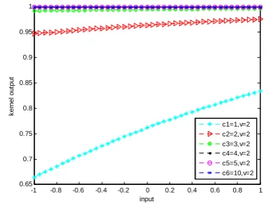
Figure 3 is a graph at the test point of 0.1when vin the
sigmoid kernel function has the value of 2 and c in the
sigmoid kernel function has different values. From the Figure3 we can see that the sigmoid kernel function has
better results and generalization ability whenc≥4, and
the output values reach a steady state.
If we further analyze the Figure 3, we can know whether the data points near the test data point or not can
have an effect on the sigmoid kernel function, but at the test point its learning ability is relatively poor. After
several experiments, we conclude that vwith the value of
2 is more appropriate.
Gaussian radial basis kernel function is a common local kernel function and its expression is as following:
2
2
( , ) exp( )
2
i i
x x K x x
σ
⋅
= − (15)
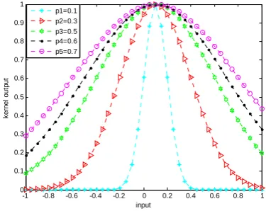
Figure 4 is a graph of Gaussian radial basis kernel
function at the test point of 0.1when σ expressed in
Figure 4 by p has different values. As it can be seen
from Figure 4, Gaussian radial basis kernel function at the test point has a strong learning ability. But its generalization ability is relatively poor, because it only allows closely spaced data points to have an effect on the kernel function. We can see from the figure 4, the parameter value and learning ability are inversely proportional. That means the greater the parameter value is, the worse its learning ability will be. After a lot of
experiments and practice, we know that the value of σ
between 0.1 and 1 is better in general.
-1 -0.8 -0.6 -0.4 -0.2 0 0.2 0.4 0.6 0.8 1 0.65
0.7 0.75 0.8 0.85 0.9 0.95 1
input
k
e
rnel
out
put
c1=1,v=2 c2=2,v=2 c3=3,v=2 c4=4,v=2 c5=5,v=2 c6=10,v=2
Figure.3 The graph of the sigmoid kernel function (v=2) at the test point of 0.1
-1 -0.8 -0.6 -0.4 -0.2 0 0.2 0.4 0.6 0.8 1 0
0.1 0.2 0.3 0.4 0.5 0.6 0.7 0.8 0.9 1
input
k
er
nel
out
put
c=1,v1=1 c=1,v2=2 c=1,v3=3 c=1,v4=4 c=1,v5=7 c=1,v6=10
-1 -0.8 -0.6 -0.4 -0.2 0 0.2 0.4 0.6 0.8 1 0
0.1 0.2 0.3 0.4 0.5 0.6 0.7 0.8 0.9 1
input
k
er
n
el
o
ut
p
ut
p1=0.1 p2=0.3 p3=0.5 p4=0.6 p5=0.7
Figure.4 The graph of Gaussian radial basis kernel function at the test
point of 0.1
III.USING THE MIXED KERNEL FUNCTION TO IMPROVE
THE TWSVM
Although there are many improved algorithms of TWSVM including optimization of parameters in kernel functions, these algorithms don’t fundamentally change the learning ability and generalization ability of the kernel functions to improve the performance of TWSVM. We take the improvement of the generalization and learning ability in the kernel function as a starting point, and then this paper proposes the twin support vector machines based on the mixed kernel function. This algorithm makes full use of the generalization ability of global kernel functions and the learning ability of local kernel functions to improve the performance of TWSVM.
A. The Mixed Kernel Function
This paper selects the sigmoid kernel function which is a common global kernel function and Gaussian radial basis kernel function which is a common local kernel function as the basic kernel functions to construct a mixed kernel function. Then it will be used to improve the performance of TWSVM. Based on this idea, we construct a function which is as following:
1 2
( , )i ( , )i ( , ),i 0, 0
K x x =aK x x +bK x x a> b> (16)
In formula (16),K x x1( , )i is the sigmoid kernel function
and K x x2( , )i is Gaussian radial basis kernel function.
The next, let us prove that this mixed function is an admissible kernel function.
Proof: According to the above-mentioned formula (9),
1( , )i
aK x x with a>0is an admissible kernel function.
Similarly, bK x x2( , )i with b>0 is an admissible kernel function. Let K x x3( , )i =aK x x where a1( , )i >0 and
4( , )i 2( , )i 0
K x x =bK x x where b> , then both
3( , )i
K x x and K x x4( , )i are admissible kernel functions.
LetK x x5( , )i =K x x3( , )i +K x x4( , )i , then according to the
above-mentioned formula (8), K x x5( , )i is an admissible
kernel function. K x x5( , )i is just the K x x( , )i . Therefore,
1 2
( , )i ( , )i ( , )i 0 0
K x x =aK x x +bK x x with a> and b> is an
admissible kernel function. QED.
aandbin the formula (16) represent the percentages of
the sigmoid kernel function and Gaussian radial basis kernel function in the mixed kernel function. In order to ensure that the mixed kernel function does not change the reasonableness of the original mapping, generally, let
0 , 1≤a b≤ anda b+ =1[23]. According to this, the formula (16)
can be converted to:
1 2
( , )i ( , ) (1i ) ( , ) 0i 1
K x x =λK x x + −λK x x ≤ ≤λ (17)
In formula (17), K x x1( , )i is the sigmoid kernel function
and K x x2( , )i is Gaussian radial basis kernel function.
Therefore, the final mathematical expression of the mixed kernel function is as following:
2 2
( , ) tanh( ( ) ) (1 )exp( ) 0 1 2
i
i i
x x
K x x λ ν x x c λ λ
σ ⋅
= ⋅ + + − − ≤ ≤ (18)
Let s=1/ 2σ2then the formula (18) can be converted
to:
2
( , )i tanh( ( i) ) (1 )exp( i ) 0 1 K x x =λ ν x x⋅ + + −c λ − ⋅ ⋅s x x ≤ ≤λ
(19) Figure 5 is a graph of the mixed kernel function at the
test point of 0.1 when ν =2 ,c=10and λ has different
values. a in the Figure 5 represents the parameter λ in
the mixed kernel function. It can be seen from the Figure 5 that the generalization ability and learning ability of the
mixed kernel function will be different when λ has
different values which means that the percentage of the sigmoid kernel function and Gaussian radial basis kernel function changes. The generalization ability of the mixed kernel function will be enhanced when the value of
λ increases. For different data sets,λwill have different
values to achieve the best results.
B. The Description of MK-TWSVM
MK-TWSVM is described as follows:
Step1 Import the data sets and divide these data sets
into two randomly. One is 80% of the data, and the other is 20%.
Step 2 Set the parameters in the sigmoid kernel
function and initialize the algorithm.
-1 -0.8 -0.6 -0.4 -0.2 0 0.2 0.4 0.6 0.8 1 0
0.1 0.2 0.3 0.4 0.5 0.6 0.7 0.8 0.9 1
input
k
er
nel
out
put
a1=0.1 a2=0.2 a3=0.4 a4=0.6 a5=0.7 a6=0.8
Step 3 Take the 80% of the data for training and
determine the value of λin the mixed kernel function,
the value of σin Gaussian radial basis kernel function
and the value of
c
1 、c
2 in TWSVM by the gridsearching method.
Step 4 Calculate the classification accuracy with the
parameter values from Step 3.
Step 5 Determine whether it is the global optimum
accuracy. If it is the global optimum accuracy, update the global optimum value and record this optimal parameter values. If it is not the global optimum accuracy, Jump to
the Step 6.
Step 6 Determine whether it reaches the end condition
of the grid cycle. If it does not, Jump to the Step 3. If it
does, Jump to the Step 7.
Step 7 Bring the optimal parameters from the training
into TWSVM. And then the final model of MK-TWSVM is determined.
Step 8 After the model of MK-TWSVM is determined,
take the remaining 20% of the data for testing to get the test classification accuracy.
Step 9 Stop operations.
The flow chart of MK-TWSVM is shown in Figure 6. By this flow chart, we can intuitively understand the process of MK-TWSVM proposed by this paper. And the nine steps of the algorithm described above are clearly expressed in Figure 6. This will help us understand the algorithm.
IV.ANALYSIS OF THE EXPERIMENTAL RESULTS
This paper selects five common data sets in the UCI machine learning database to test and validate the algorithm proposed by us. The 80% of the data will be used for training and the remaining 20% of the data will be used for testing. Since we want to verify that the mixed kernel function proposed by this paper will improve the performance of TWSVM, we only do the nonlinear experiments. The five data sets are ionosphere data set, Sonar data set, votes data set, bupa data set and Hepatitis data set. Using the MATLAB environment, we do these experiments on a PC. In this algorithm, the value
of vin the sigmoid kernel function is 2 and the value of
c in the sigmoid kernel function is 10. We will get the
optimal values of λ in the mixed kernel function, sin
Gaussian radial basis kernel function and c c1, 2 in
TWSVM through grid computing. For different data sets, their values are different.
The used data sets are sonar data set, ionosphere data set, Votes data set, bupa data set and Hepatitis data set in these experiments. Their characteristics are shown in Table I.
TABLE I.
THE DATA CHARACTERISTICS OF THE DATA SETS
Data sets The number of samples The number of attributes
Sonar 208 60 Ionosphere 351 34
Votes 435 16 bupa 345 7 Hepatitis 155 19
In the experiments, MK-TWSVM randomly selects 80% of the data to be used for training and then it gets the optimal parameters to determine the model. Then, the remaining 20% of the data is used for testing to get the corresponding classification accuracy. We compare the experimental results of MK-TWSVM with PSVM, GEPSVM and TWSVM. The Table II shows the results of the comparison.
TABLE II THE EXPERIMENTAL RESULTS
Data sets MK-TWSVM TWSVM GEPSVM PSVM Sonar 93.02 89.64 85.97 82.79 Ionosphere 95.77 87.46 84.41 90.83
Votes 96.59 94.91 94.5 93.70
bupa 69.57 68.64 68.18 65.8
Hepatitis 82.35 81.39 79.28 78.57
In order to visually observe the experimental results, we plot the results in Figure 7. The ordinate represents the classification accuracy values. The abscissa of 1 represents the sonar data set. The abscissa of 2 represents the bupa data set. The abscissa of 3 represents the ionoshere data set. The abscissa of 4 represents the Hepatitis data set. The abscissa of 5 represents the Votes data set. The effect diagram is shown in Figure 7:
1 1.5 2 2.5 3 3.5 4 4.5 5
65 70 75 80 85 90 95 100
Sonar
Bupa
votes Ionosphere
Hepatitis
data sets
cl
a
s
s
ifi
ca
ti
o
n
a
c
cu
ra
c
y
MK-TWSVM TWSVM GEPSVM PSVM
Figure.7 The effect diagram of the comparison
We can see from the test results that the classification accuracy of MK-TWSVM proposed by this paper has increased significantly, compared with the traditional classification algorithms. In Figure 7, we can see more intuitively that the classification accuracy curve of MK-TWSVM is obviously above the classification accuracy curves of TWSVM, GEPSVM and PSVM. It means that the classification accuracy of MK-TWSVM is better than theirs and has significantly improved. Why can it be able to achieve such a significant effect? It is because that MK-TWSVM has used the mixed kernel function. The mixed kernel function does not randomly select any kernel functions to be combined, but selects a global kernel function and a local kernel function to be combined. The global kernel function has a good generalization ability and the local kernel function has a good learning ability. MK-TWSVM adjusts the proportion of the global kernel function and the local
kernel function through adjusting the value ofλ to further
make the learning ability and generalization ability achieve an optimum balance. We can see from this analysis that the biggest improvement of MK-TWSVM is the introduction of the mixed kernel function. And it makes full use of the advantages of the global and local kernel functions to improve the performance of TWSVM.
V.CONCLUSIONS
In recent years, classification algorithms have various improvements and TWSVM also has been developed rapidly. But TWSVM still has many defects, such as the problem of selecting the kernel function. For this problem, we propose the MK-TWSVM in this paper. It makes full use of the generalization ability of global kernel functions and the learning ability of local kernel functions and then it achieves an optimum balance between them to further determine the model of MK-TWSVM. This avoids the case that the traditional TWSVM only uses a single kernel function. In that case, there exists a problem. If it selects a global kernel function, its generalization ability is good, but the learning ability is relatively weak. If it selects a local kernel function, its learning ability is good, but the generalization ability is relatively weak. Therefore,
kernel function to construct a mixed kernel function which has the better performance. And then MK-TWSVM introduces it into MK-TWSVM. So MK-MK-TWSVM can make full use of their respective advantages to improve the performance of TWSVM.
The experiments show that MK-TWSVM improves the classification accuracy of TWSVM. But MK-TWSVM also has a defect that the parameters are difficult to be determined. In addition to the parameters of TWSVM, there are parameters of the mixed kernel function. So MK-TWSVM relatively has more parameters and finds the optimal parameters more difficultly. Because of the more parameters, it will take more time. Therefore, we can start from this point in the following research work. If we can optimize the parameters, we will improve the performance of MK-TWSVM to further improve the classification efficiency and accuracy of TWSVM.
REFERENCES
[1] CRISTIANINI N,TAYLOR J S. An introduction to
support vector machines and other kernel-based learning methods. Translated by Li Guozheng ,Wang Meng,Zeng Huajun.Beijing: Electronic Industry Press, 2004.
[2] Ding Shifei, Qi Bingjuan, Tan Hongyan. An Overview on
Theory and Algorithm of Support Vector Machines. Journal of University of Electronic Science and Technology of China, 2011, 40(1):2-10.
[3] C.Cortes,V.Vapnik. Support-Vector Networks. Maching
Learning,1995,20(2), 273-297.
[4] Vapnik V N. The nature of statistical learning theory.
Translated by Zhang Xuegong.Beijing: Tsinghua University Press, 2000.
[5] Vapnik V.N.Statical Learning Theory. Translated by Xu
Janhua, Zhang Xuegong. Beijing: Electronic Industry Press, 2004.
[6] Masaki Murata, Tomohiro Mitsumori, Kouichi Doi.
Analysis and Improved Recognition of Protein Names Using Transductive SVM. Journal of Computers,2008,3(1), 51-62.
[7] Lianwei Zhang, Wei Wang, Yan Li, Xiaolin Liu, Meiping
Shi, Hangen He . A Method for Surface Reconstruction Based on Support Vector Machine. Journal of Computers,2009,4(9), 806-812.
[8] Qisong Chen, Xiaowei Chen, Yun Wu. Optimization
Algorithm with Kernel PCA to Support Vector Machines for Time Series Prediction. Journal of Computers,2010,5(3), 380-387.
[9] Wei Liu, Yuhua Yan, Rulin Wang.Application of
Hilbert-Huang Transform and SVM to Coal Gangue Interface Detection. Journal of Computers,2011,6(6), 1262-1269.
[10]Lei Zhang, Yanfei Dong.Research on Diagnosis of AC
Engine Wear Fault Based on Support Vector Machine and Information Fusion. Journal of Computers,2012,7(9), 2292-2297.
[11]Lei Ding, Fei Yu, Sheng Peng, Chen Xu.A Classification
Algorithm for Network Traffic based on Improved Support Vector Machine. Journal of Computers,2013,8(4),1090-1096.
[12] J.A.K. SUYKENS, J. VANDEWALLE. Least Squares
Support Vector Machine Classifiers. Neural Processing Letters ,1999,9:293–300.
[13]Fung G, Mangasarian O L. Proximal support vector
machine classifiers. In: Proc 7th ACMSIFKDD Intl Conf on Knowledge Discovery and Data Mining, 2001: 77-86.
[14]Mangasarian Olvi L, Wild Edward W. Multisurface
proximal support vector machine classification via generalized eigenvalues.IEEE Transactions on Pattern Aalysis and Machine Intelligence, 2006, 28(1): 69-74.
[15]Li Kai, Lu Xiao Xia. Twin Support Vector Machine
Algorithm with Fuzzy Weighting. Computer Engineering and Applications.2011.
[16]Jayadeva, Khemchandni Reshma, Suresh Chandra. Twin
support vector machines for pattern classification. IEEE Transactions on Pattern Analysis and Machine Intelligence, 2007, 29(5):905-910.
[17]Ding Shifei, Yu Junzhao, Qi Bingjuan. An Overview on
Twin Support Vector Machines. Artificial Intelligence Review, 2012 (DOI:10.1007/s10462-012-9336-0).
[18]Junzhao Yu, Shifei Ding, Fengxiang Jin, Huajuan Huang,
Youzhen Han. Twin Support Vector Machines Based on Rough Sets. International Journal of Digital Content Technology and its Applications, 2012, 6(20):493-500.
[19]Chen Jing, Ji Guangrong. Weighted least squares twin
support vector machines for pattern classification. 2010 The 2nd International Conference on Computer and Automation Engineering, Singapore: [s.n.], 2010, 2:242-246.
[20]Qi Zhiquan, Tian Yingjie, Shi Yong. Robust twin support
vector machine for pattern classification. Pattern Recognition. 2013, 46(1):305-316.
[21]Xinsheng Zhang, Xinbo Gao, Ying Wang.MCs Detection
with Combined Image Features and Twin Support Vector Machines. Journal of Computers,2009,4(3), 215-221.
[22]Huajuan Huang, Shifei Ding, Fengxiang Jin, Junzhao Yu,
Youzhen Han. A Novel Granular Support Vector Machine Based on Mixed Kernel Function. International Journal of Digital Content Technology and its Applications, 2012, 6(20):484-492.
[23]Wang Guosheng. Properties and Construction Methods of
Kernel in Support Vector Machine. Computer Science,2006,33(6): 172-174.
Fulin Wu is currently a graduate student
now studying in School of Computer Science and Technology, China University of Mining and Technology, and his supervisor is Prof. Shifei Ding. He received his B.Sc. degree in computer science from China University of Mining and Technology in 2012. His research interests include cloud computing, feature selection, pattern recognition, machine learning et al.
Shifei Ding is a professor and Ph.D.