Enhancement of Power Transfer Capability of Interconnected Power System by Using FACTS Controllers with OPF Method

www.ijres.org Volume 6 Issue 5 Ver. I ǁ 2018 ǁ PP. 62-72

Enhancement of Power Transfer Capability of Interconnected

Power System by Using FACTS Controllers with OPF Method

M.Sheshagiri

, Dr.B.V.Sankerram

1_{(TSTRANSCO,Vidyut Soudha,Hyderabad,Telangana,India)}

2_{( Department of EEE,College of Engineering,JNTUH,Kukatpally,Hyderabad,Telangana,India)}

Corresponding Author: M.Sheshagiri

Abstract :

Keywords -

--- --- Date of Submission: 15-06-2018 Date of acceptance: 30-06-2018 --- ---

I. INTRODUCTION

Transmission open access has been an important issue in the ongoing deregulation and restructuring of power sector in many countries. Transmission open access is a vehicle for promoting competition in generation. Open access to the transmission systems places a new emphasis on the more intensive shared use of the interconnected networks reliably by utilities and third party generators. As system becomes deregulated, loop networks introduced technical issues with the definition and calculation of the ATC. In addition, the differences between contract path and actual power flow path introduced additional complexity to the quantification of ATC. When systems were isolated and largely radial, these capabilities were fairly easy to determine and consisted mainly of a combination of thermal ratings and voltage drop limitations. In most cases, these two limitations were easily combined into a single power limitation (either MW or MVA or surge impedance loading). As such, ATC for a given transmission line at a given time could be interpreted as the difference between the power limit and the power flow at that time. Owing to the commercial and technological significance of ATC in the power industry deregulated environment, more and more institutes and utilities have shown increased interest and are undertaking studies of evaluation and enhancement of ATC. In recent years various approaches have been proposed to modal and calculate ATC. Under open access power system complexity has grown and system stabilities became an important constraint for some areas of the interconnected network and this required the consideration of the third limiting phenomena. The introduction of St. Clair curves were one of the first attempts to include thermal, voltage and stability into a single transmission line loading. These results were later verified and extended from a more theoretical basis. Linear load flow and linear programming solutions made transmission transfer capability determination relatively fast and easy. It is highly recognized that flexible AC transmission systems (FACTS) devices, specially the series devices such as thyristor controlled series capacitor (TCSC), thyristor controlled phase angle regulator (TCPAR), unified power flow controller (UPFC) etc. can be applied to increase the ATC of power network. In [1] a comparative study to improve ATC has been done and it is shown that FACTS technology can redistribute load flow and regulate bus voltage, so a promising method to improve TTC. In [9] location of FACTS devices has been suggested with increase in total transfer capability.

II. FACTSDEVICES

1.1 Selection of Devices

FACTS devices are categorized under four different categories as series controllers, shunt controllers, combined series and shunt controllers. In this paper, one device from each category is selected i.e., TCSC from series controllers, SVC from shunt controllers and UPFC from combined series-shunt controllers. TCSC is connected in series with the line conductors to compensate for the inductive reactance of the line. It may have one of the two possible characteristics namely capacitive or inductive, respectively to decrease or increase the reactance of the line XL respectively. Moreover, in order not to overcompensate the line, the maximum value of the capacitance is fixed at - 0.8 XL while that for inductance, it is 0.2 XL. Although TCSC is not usually installed for voltage control purpose, it does contribute for better voltage profile and reactive power control. SVC is used for voltage control applications. It helps to maintain a bus voltage at a desired value during load variations. The SVC may have two characteristics namely, inductive or capacitive. In the inductive mode, it absorbs reactive power, whereas in the capacitive mode, reactive power is injected. It may take values characterized by the reactive power injected or absorbed at the voltage of 1 p.u.

The values are between -100 Mvar and 100 Mvar. The UPFC is capable of providing active and reactive power control, as well as adaptive voltage magnitude control and regulates all the three variables simultaneously or any combination of them, provided no operating limits are violated. The UPFC may act as an SVC, a TCSC or a phase shift controller. The versatility afforded by the UPFC makes it a prime contender to provide many of the control functions required to solve a wide range of dynamic and steady state problems encountered in electrical power networks [9]. UPFC can be modeled as a combination of one series element i.e., TCSC and a shunt element i.e., SVC [3]. Hence the operational range limits of TCSC and SVC can be applied to UPFC as well.

2.2 Modeling of FACTS Devices

TCSC has been modeled as a variable reactance inserted in the transmission line connected between buses. SVC is modeled as a reactive power source added or connected at the bus. Based on previous research [2], UPFC is modeled as combination of an SVC at a bus and a TCSC in the line connected to the same bus.

2.3 Device Placement Strategy

ATC value is greatly influenced by the power flow in the limiting line of the system. Therefore, a FACTS device is placed in the limiting line or at the corresponding bus to which the limiting line is connected depending on the type of device. Only one FACTS device per line is allowed. If only one device is used, it is placed in the first limiting line of the system. If three devices are to be inserted, then the first three limiting lines are selected. For this purpose, the limiting lines in the considered test systems are ranked and ordered based upon the power carrying capacity in the line. For the multi-type device category, TCSC is considered as the first device, SVC as the second and UPFC as the third. If the device is TCSC, it is connected in series with the limiting line. If the device is SVC, then the type of originating bus and terminating bus of the limiting line is checked. If the one end bus is PV bus, it is discarded and if the other end bus is PQ bus, then SVC is connected. Suppose if two end buses happen to be PV buses, then the next limiting line in the order is selected and checked for type of bus. For UPFC, the series device TCSC is connected in series with the limiting line and the shunt device SVC is connected at PQ bus after checking the type of the end buses where the limiting line is connected.

III. OPTIMALPOWERFLOWMETHOD

In an OPF, the values of some or all of the control variables need to be found so as to optimize (minimize or maximize) a predefined objective. It is also important that the proper problem definition with clearly stated objectives be given at the onset. The quality of the solution depends on the accuracy of the model studied. Objectives must be modeled and its practicality with possible solutions. Objective function takes various forms such as fuel cost, transmission losses and reactive source allocation. Usually the objective function of interest is the minimization of total production cost of scheduled generating units. This is most used as it reflects current economic dispatch practice and importantly cost related aspect is always ranked high among operational requirements in Power Systems. OPF aims to optimize a certain objective, subject to the network power flow equations and system and equipment operating limits. The optimal condition is attained by adjusting the available controls to minimize an objective function subject to specified operating and security requirements. Some well-known objectives can be identified as below:

Active power objectives

1. Economic dispatch (minimum cost, losses, MW generation or transmission losses)

2. Environmental dispatch 3. Maximum power transfer Reactive power objectives MW and MVAr loss minimization.

General goals

1. Minimum deviation from a target schedule 2. Minimum control shifts to alleviate Violations

3. Least absolute shift approximation of control shift Among the above the following objectives are most commonly used: (a) Fuel or active power cost optimization (b) Active power loss minimization (c) VAr planning to minimize the cost of reactive power support The mathematical description of the OPF problem is presented below: OPF Objective Function for Fuel Cost Minimization The OPF problem can be formulated as follows:

Total Generation cost function is expressed as:

F(PG) = ∑(ai +βPGi+PGi2)

The objective function is expressed as: Min F(PGi) = f(x,u)

Subject to satisfaction of Non-Linear Equality Constraints:

G(x,u) = 0

And Non Linear Inequality Constraints: H(x,u)0

uminuumax xminxxmax

IV. SIMULATION MODEL AND RESULTS

MATLAB (short for MATrix LABoratory) is a special purpose computer program optimized to perform engineering and scientific calculations. It started life as a program designed to perform matrix mathematics, but over the years it has grown into a flexible computing system capable of solving essentially any technical problem.

A MATLAB program provides a very extensive library of predefined functions to make technical programming tasks easier and more efficient. It is a huge program, with an incredibly rich variety of functions. It has an extensive library of built-in functions for data manipulation and the toolkits extend this capability with many more functions in various specialties. MATLAB comes complete with a library of pre-programmed and tested models, ranging from simple passive elements and control functions, to more complex models, such as FACTS devices.

Optimal Power Flow method:

 Considered 14-bus and 30-bus systems for enhancement of power transfer capability.

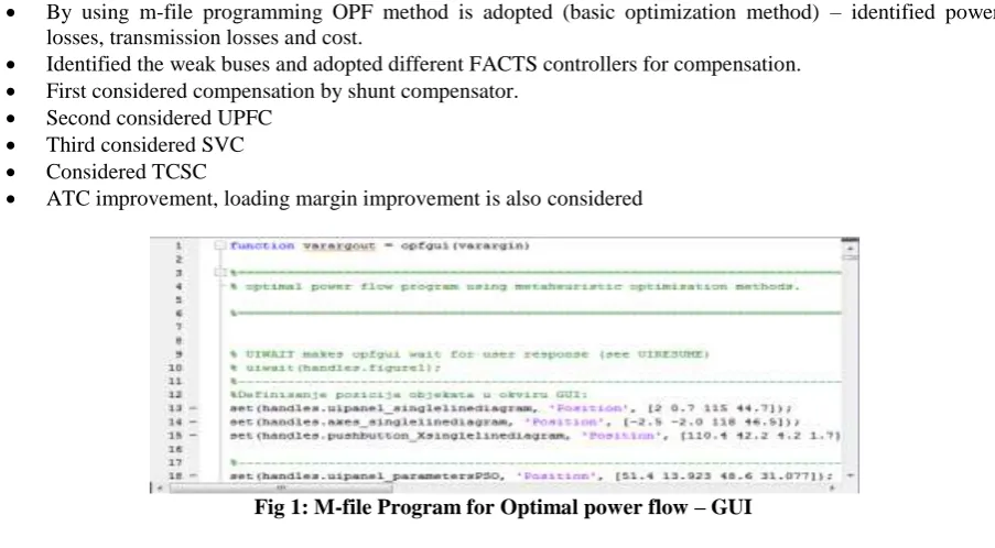
 By using m-file programming OPF method is adopted (basic optimization method) – identified power losses, transmission losses and cost.

 Identified the weak buses and adopted different FACTS controllers for compensation.

 First considered compensation by shunt compensator.

 Second considered UPFC

 Third considered SVC

 Considered TCSC

 ATC improvement, loading margin improvement is also considered

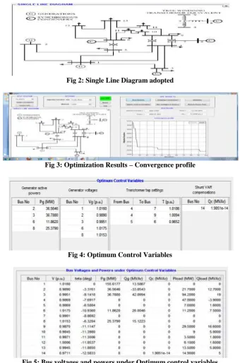
Fig 2: Single Line Diagram adopted

Fig 3: Optimization Results – Convergence profile

Fig 4: Optimum Control Variables

Fig 5: Bus voltages and powers under Optimum control variables

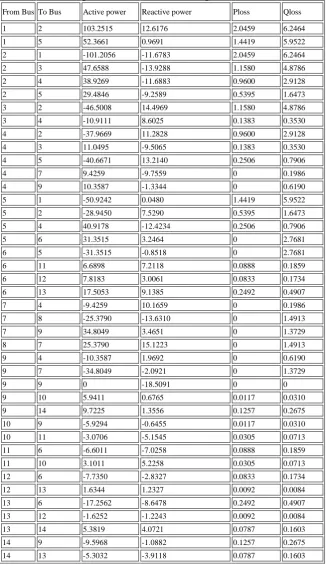
Table 1: Branch power flow and Loss under optimum control variables

From Bus To Bus Active power Reactive power Ploss Qloss

1 2 103.2515 12.6176 2.0459 6.2464

1 5 52.3661 0.9691 1.4419 5.9522

2 1 -101.2056 -11.6783 2.0459 6.2464

2 3 47.6588 -13.9288 1.1580 4.8786

2 4 38.9269 -11.6883 0.9600 2.9128

2 5 29.4846 -9.2589 0.5395 1.6473

3 2 -46.5008 14.4969 1.1580 4.8786

3 4 -10.9111 8.6025 0.1383 0.3530

4 2 -37.9669 11.2828 0.9600 2.9128

4 3 11.0495 -9.5065 0.1383 0.3530

4 5 -40.6671 13.2140 0.2506 0.7906

4 7 9.4259 -9.7559 0 0.1986

4 9 10.3587 -1.3344 0 0.6190

5 1 -50.9242 0.0480 1.4419 5.9522

5 2 -28.9450 7.5290 0.5395 1.6473

5 4 40.9178 -12.4234 0.2506 0.7906

5 6 31.3515 3.2464 0 2.7681

6 5 -31.3515 -0.8518 0 2.7681

6 11 6.6898 7.2118 0.0888 0.1859

6 12 7.8183 3.0061 0.0833 0.1734

6 13 17.5053 9.1385 0.2492 0.4907

7 4 -9.4259 10.1659 0 0.1986

7 8 -25.3790 -13.6310 0 1.4913

7 9 34.8049 3.4651 0 1.3729

8 7 25.3790 15.1223 0 1.4913

9 4 -10.3587 1.9692 0 0.6190

9 7 -34.8049 -2.0921 0 1.3729

9 9 0 -18.5091 0 0

9 10 5.9411 0.6765 0.0117 0.0310

9 14 9.7225 1.3556 0.1257 0.2675

10 9 -5.9294 -0.6455 0.0117 0.0310

10 11 -3.0706 -5.1545 0.0305 0.0713

11 6 -6.6011 -7.0258 0.0888 0.1859

11 10 3.1011 5.2258 0.0305 0.0713

12 6 -7.7350 -2.8327 0.0833 0.1734

12 13 1.6344 1.2327 0.0092 0.0084

13 6 -17.2562 -8.6478 0.2492 0.4907

13 12 -1.6252 -1.2243 0.0092 0.0084

13 14 5.3819 4.0721 0.0787 0.1603

14 9 -9.5968 -1.0882 0.1257 0.2675

14 13 -5.3032 -3.9118 0.0787 0.1603

IEEE 30-Bus System with FACTS Compensators:

Fig 7: Single line diagram of IEEE 30 bus system

Fig 8: Simulation model of IEEE 30-bus system

--- 25 1.0032 -16.0720 26 0.9852 -16.5038 30 0.9828 -17.8067

Fig 9: Weakest Buses obtained before compensation for IEEE 30 bus system

FACTS controllers placed at 30 Bus system

Fig 10: Voltage improvement with FACTS controller in IEEE 30 bus system

Analysis without FACTS controllers for IEEE 14 Bus system:

From the Optimal power flow the weak buses with power losses are identified for inter and intra buses. From Bus To Bus Active power Reactive power Ploss Qloss

1 2 103.2515 12.6176 2.0459 6.2464 1 5 52.3661 0.9691 1.4419 5.9522 2 1 -101.2056 -11.6783 2.0459 6.2464 3 2 -46.5008 14.4969 1.1580 4.8786 5 1 -50.9242 0.0480 1.4419 5.9522

Continuous

powergui

ABC

abc ABC

abc

ABC

abc ABC

abc ABC

abc ABC

abc

A BC A BC ABC ABC AB C AB C A BC A BC A BC A BC AB C AB C ABC ABC A BC A BC A BC A BC A BC A BC AB C ABC A BC A BC A B C A BC A BC A BC AB C AB C A BC A BC A BC A BC A BC A BC A BC A BC A BC A BC A BC A BC ABC ABC A BC A BC AB C AB C AB C AB C A BC A BC ABC ABC AB C AB C A BC A BC A BC A BC A BC A BC AB C AB C AB C AB C ABC ABC ABC ABC A BC A BC AB C AB C A BC A BC AB C AB C AB C AB C A BC A BC ABC ABC Sw Pulses A B C VdcP N VdcM Shunt Converter 500 kV, 100MVA

PulsesA1 B1 C1 A2 B2 C2 VdcP N VdcM Series Converter 10% injection, 100MVA Scope9 Scope8 Scope7 Scope60 Scope6 Scope59 Scope58 Scope57 Scope56 Scope55 Scope54 Scope53 Scope52 Scope51 Scope50 Scope5 Scope49 Scope48 Scope47 Scope46 Scope45 Scope44 Scope43 Scope42 Scope41 Scope40 Scope4 Scope39 Scope38 Scope37 Scope36 Scope35 Scope34 Scope33 Scope32 Scope31 Scope30 Scope3 Scope29 Scope28 Scope27 Scope26 Scope25 Scope24 Scope23 Scope22 Scope21 Scope20 Scope2 Scope19 Scope18 Scope17 Scope16 Scope15 Scope14 Scope13 Scope12 Scope11 Scope10 Scope1

VabcAIabcBabCcBUS9

VabcAIabcBabCcBUS8

VabcAIabcBabCcBUS7

VabcAIabcBabCcBUS6

VabcAIabcBabCcBUS5

VabcAIabcBabCcBUS4

VabcAIabcBabCcBUS30

VabcAIabcBabCcBUS3

VabcAIabcBabCcBUS29

VabcAIabcBabCcBUS28

VabcAIabcBabCcBUS27

VabcAIabcBabCcBUS26

VabcAIabcBabCcBUS25

VabcAIabcBabCcBUS24

VabcAIabcBabCcBUS23

VabcAIabcBabCcBUS22

VabcAIabcBabCcBUS21

VabcAIabcBabCcBUS20

VabcAIabcBabCcBUS2

VabcAIabcBabCcBUS19

VabcAIabcBabCcBUS18

VabcAIabcBabCcBUS17

VabcAIabcBabCcBUS16

VabcAIabcBabCcBUS15

VabcAIabcBabCcBUS14

VabcAIabcBabCcBUS13

VabcAIabcBabCcBUS12

VabcAIabcBabCcBUS11

VabcAIabcBabCcBUS10

VabcAIabcBabCcBUS1

VabcIabc PQ VabcIabc PQ VabcIabc PQ VabcIabc PQ VabcIabc PQ VabcIabc PQ VabcIabc PQ VabcIabc PQ VabcIabc PQ VabcIabc PQ VabcIabc PQ VabcIabc PQ VabcIabc PQ VabcIabc PQ VabcIabc PQ VabcIabc PQ VabcIabc PQ VabcIabc PQ VabcIabc PQ VabcIabc PQ VabcIabc PQ VabcIabc PQ VabcIabc PQ VabcIabc PQ VabcIabc PQ VabcIabc PQ VabcIabc PQ VabcIabc PQ VabcIabc PQ VabcIabc PQ abc Mag Phase abcMag Phase abc Mag Phase abc Mag Phase abc Mag Phase abcMag Phase abc Mag Phase abc Mag Phase abc Mag Phase abcMag Phase abc Mag Phase abc Mag Phase abcMag Phase abcMag Phase abc Mag Phase abc Mag Phase abc Mag Phase abcMag Phase abcMag Phase abc Mag Phase abcMag Phase abc Mag Phase abcMag Phase abc Mag Phase abc Mag Phase abc Mag Phase abc Mag Phase abc Mag Phase abcMag Phase abcMag Phase

ABC

Gen6

ABC

Gen5

ABC

Gen4

ABC

Gen3

ABC

Gen2

ABC

Gen1

ABC

R Load 9

ABC

R Load 8

ABC

R Load 7

ABC

R Load 6

ABC

R Load 5

ABC

R Load 4

ABC

R Load 3

A B C R Load 26

ABC

R Load 25

ABC

R Load 24

AB C

R Load 23

ABC

R Load 22

ABC

R Load 21

ABC

R Load 20

ABC

R Load 2

ABC

R Load 18

ABC

R Load 17

AB C

R Load 16

ABC

R Load 15

AB C

R Load 14

ABC

R Load 13

ABC

R Load 12

ABC

R Load 11

ABC

R Load 10

ABC

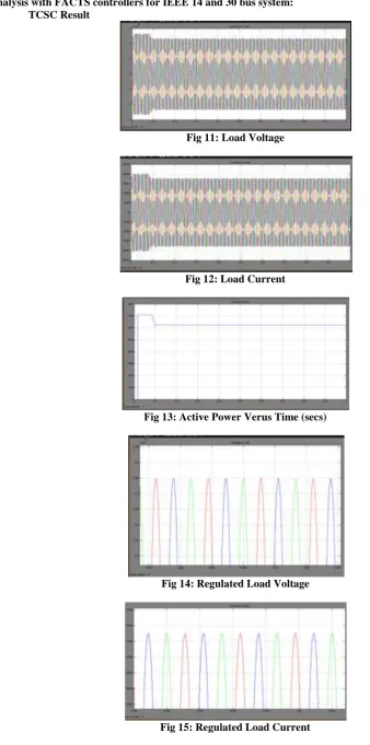
Analysis with FACTS controllers for IEEE 14 and 30 bus system:

a) TCSC Result

Fig 11: Load Voltage

Fig 12: Load Current

Fig 13: Active Power Verus Time (secs)

Fig 14: Regulated Load Voltage

Fig 16: Regulated Load Power

b) UPFC Result:

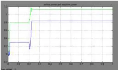
Fig 17: Subsystem of 14-bus system with UPFC

Fig 18: Active and Reactive Power Versus Time (Secs) C ontinuous powe rgui v + -Voltage Measurement8 v + -Voltage Measurement3 v+ -Voltage Measurement2 v+ -Voltage Measurement g m a k Thyristor7 g m a k Thyristor6 g m a k Thyristor5 g m a k Thyristor4 g m a k Thyristor3 g m a k Thyristor2 g m a k Thyristor1 g m a k Thyristor Scope6 Scope21 Scope20 Scope2 Scope19 Scope18 Scope17 Scope16 Scope14 Scope13 Scope1 Pul se Generator8 Pul se Generator7 Pul se Generator6 Pul se Generator5 Pul se Generator4 Pul se Generator3 Pul se Generator2 Pul se Generator1 Load 2 Load 1 1 2 Line 9 1 2 Line 1 P1 P2 P3 P4 IEEE14BUSSYST EM G2 i + -C urrent Measurement3

Breaker V IP Q Active & Reactive

Power3

Bus1 Bus 2 Li ne 1

Li ne 5 Li ne 2

Bus 5

Li ne 6 Li ne 4

Li ne 3

Bus 4

Bus 3 Li ne 7 Bus 6

Bus 13 Bus 14

Bus 9 Bus 10 Bus 11 Bus 12

Li ne 16 Li ne 11

Li ne 12 Li ne 13

Li ne 17

Li ne 18 Li ne 19 Li ne 20

Bus 7 Bus 8 4 P4 3 P3 2 P2 1 P1 v + -Voltage Measurement4

v+

-Voltage Measurement3 v + -Voltage Measurement1 Scope9 Scope3 Scope12 Scope11 Scope1 Load 9 Load 7 Load 6 Load 5 Load 3 Load 14 Load 13 Load 12 Load 11 Load 1 1 2 Line 9 1

2 Line 15

1 2 Line 14 1 2 Line 10 1 2 Line 1 L9 L7 L6 L5 L4 L3 L2 L17 L16 L15 L14 Line 17 L13 L11 L10 L1 G1 i

+-C urrent Measurement3

i

+-C urrent Measurement1

C ondenser1

C 3 C

V

I P Q

Active & Reactive Power3

V

I P Q

Fig 19: Load Voltage – 1 & 2

Fig 20: DC capacitor Voltage

c) SVC Controller:

Fig 21: Simulation model with SVC output controller

Fig 22: Three Phase Voltages Versus Time (secs)

Fig 23: Three Phase Currents Versus Time (secs)

Enhancement of power transfer capability IEEE 14 Bus System:

Q

<---Compensated T ransmission Lines Out1 Conn1 Conn2 weak system A B C a b c relay Discrete, Ts = 5e-005 s.

Subsystem A B C a b c Secondary (16 kV)1 A B C a b c Secondary (16 kV) Scope4 Scope3 Scope2 Scope1 Vabc_prim Vabc_sec TCR TSC1 TSC2 TSC3 SVC Controller

In1In2In3In4

C onn1 C onn2 C onn3 C onn4 C onn5 C onn6 SVC A B C a b c Primary (735 kV)3 A B C a b c Primary (735 kV)2 A B C a b c Primary (735 kV)1 A B C a b c Primary (735 kV) Load Vabc_Prim33 From3 Iabc_Prim33 From2 Vabc_Prim Vabc_Sec

ABC ABC

Fault Breaker In RMS Discrete RMS value A B C AREA 4 A B2 C AREA 3 A B C AREA 2 A B C AREA 1 A B C A B C 735kV 100 MVA 3 A B C A B C 735kV 100 MVA 2

A B C A B C 735kV 100 MVA 1

A B C A B C 735kV 100 MVA

A B C a b c 735/230kV 333 MVA1 A B C a b c 735/230 kV 100 MVA

ABC

200 MW1

ABC

200 MW

Line2

Line11

From Area To Area TTC (MW) Constraint

Without FACTS devices 1 2 26

No Reactive power Limits

FACTS devices (TCSC) 34.2

Violating reactive power limit of generator at bus: 1;

FACTS devices (UPFC) 36

FACTS devices (SVC) 28

From Area To Area TTC(MW) Constraint

Without FACTS devices 1 5 31 No Reactive power Limits

FACTS devices (TCSC) 39

Violating reactive power limit of generator at bus: 5;

FACTS devices (UPFC) 43

FACTS devices (SVC) 35

From Area To Area TTC(MW) Constraint

Without FACTS devices

3 2

38.6 No Reactive power Limits

FACTS devices (TCSC) 39.1

Violating reactive power limit of generator at bus: 3;

FACTS devices (UPFC) 44

FACTS devices (SVC) 38.2

Enhancement of power transfer capability IEEE 30 Bus System

Transfer OPF method

From Area To Area TTC(MW) Constraint

Without FACTS devices

29 30

115.9

No Reactive power Limits

FACTS devices(TCSC) 115.1

Violating reactive power limit of generator at bus: 30;

FACTS devices(UPFC) 168.1

FACTS devices(SVC) 107.5

From Area To Area TTC(MW) Constraint

Without FACTS devices

25 26

115.9

No Reactive power Limits

FACTS devices(TCSC) 117.729

Violating reactive power limit of generator at bus: 30;

FACTS devices(UPFC) 149.2

FACTS devices(SVC) 110.228

V. CONCLUSION

These simulation results gives us a clear idea about the use of FACTs controllers on the interconnection of two different power system in order to maximize the real and reactive power flow between them. The FACTs devices are capable to control the real and reactive power as well as the line impedance, phase angle and voltage magnitude. From the results it is clear that UPFC able to control the flow of active power better than other two controllers (SVC and TCSC) and enhances TTC.

REFERENCES

[1]. M. Karthikeyan, P. Ajay-D-Vimalraj “Optimallocation of shunt FACTS devices for power flow control” IEEE proceeding of ICETECT 2011,pp 154-159.

[2]. M. Kowsalya, K.K. Ray, and D.P. Kothari, „Positioningof SVC and STATCOM in a Long Transmission Line‟ International Journal of Recent Trends in Engineering, Vol 2, No. 5, November 2009.

[3]. Tan, Y.L., “Analysis of line compensation by shunt connected FACTS controllers: a comparison between SVC and STATCOM”,

IEEE Transactions on PowerEngineering Review, Vol.19, pp 57-58, Aug 1999.

[5]. A.A Edris „„Enhancement of first swing stabilityusing a high speed phase shifter” IEEE Tran. on power system, Vo1.6, L991,pp I I1:LI 118.

[6]. Kimbark E W "How to improve system stabilitywithout risking sub synchronous resonance '' IEEE Tran.1977, PAS-96(s), pp 1608-1619.

[7]. M H Haque “Optimal location of shunt FACTS devices in long transmission line" IEEE Proceeding. Generation. Transmission & Distribution. Vol. 147, No.4, July 2000.

[8]. Schauder, C, Gernhardt M. Staev E, Lemark, T.Gyugyl, L. Cease T W and Edris, A " Development of a +100MVAR static condenser for voltage control of transmission system" IEEE Tran. 1995, PD-IO (3),pp 1486-1496

[9]. Chandrakar, V.K. Kothari, A.G. “Optimal location for line compensation by shunt connected FACTS controller”, The Fifth International IEEE Conference on PowerElectronics and Drive Systems”, Vol 1, pp 151 -156, Nov 2003.

[10]. Nimit Boonpirom, Kitti Paitoonwattanakij, „Static Voltage Stability Enhancement using FACTS‟ IEEE/PES transmission and distribution Conference and ExhibitionAsia Pacific., pp.1 – 5, 2007.

[11]. P. Kundur, J. Paserba, V. Ajjarapu, G. Andersson, A.Bose, C. Canizares, N. Hatziargyriou, D. Hill, A.Stankovic, C. Taylor, T. V. Cutsem and V. Vittal, 'Definition and classification of power system stability', IEEE Trans. Power Systems, 19(2) (2004), 1387-1401 .