ANALYSIS OF VOLTAGE STABILITY AND TRANSFER CAPABILITY ENHANCEMENT OF TRANSMISSION SYSTEM USING FACTS

(1)

ANALYSIS OF VOLTAGE STABILITY AND TRANSFER

CAPABILITY ENHANCEMENT OF TRANSMISSION

SYSTEM USING FACTS CONTROLLERS

Ms. CHITRA THAKUR

Designation: Assistant Professor, Organization: TIT, BHOPAL Email ID: [email protected]

Mr. SAURABH SAHU

Designation: student, Organization: TIT, BHOPAL Email ID: [email protected]

Abstract — Power flow control, in an existing long transmission line, plays a vital role in Power System area. This paper deals with shunt connected compensation (SVC and STATCOM) based FACTS device for the control of voltage and the power flow in long distance transmission line. The device proposed here is used in different locations such as source end of the transmission line, in between and load end of the transmission line. The paper also deals with resolving of the optimal location of shunt flexible a.c. transmission system (FACTS) devices for a long transmission line for voltage and power transfer improvement. The results also show that optimal location depends upon voltage magnitude and the line loading and system initial operating conditions. In this paper the two machine 4-bus test system were

simulated using MATLAB Simulink environment.

Keyword — Stability, simulation, power transfer,

SVC.

1. I

NTRODUCTION

The flexible AC transmission system (FACTS) has received much attention in the last two decades. It uses high-current power electronic devices for stability, voltage control, power flow etc. of a transmission system. Some forms of FACTS devices are already available for prototype installation [l, 2] and others are still under development. FACTS devices can be connected to a transmission line in various ways, such as in series, shunt or a combination of series and shunt. For example, static VAr compensator (SVC) and static synchronous compensator (STATCOM) are connected in shunt; static synchronous series compensator (SSSC) and thyristor-controlled series capacitor (TCSC) are connected in series; thyristor controlled phase shifting transformer (TCPST) and unified power flow controller (UPFC) are connected in a series and shunt combination. The terms and definitions of various FACTS devices are described in a recent IEEE article [3]. FACTS devices are very effective and capable of increasing the power transfer capability of a line, if the thermal limit permits, while maintaining the same degree of stability [4-7].

This paper investigates the effects of considering the actual line model on the power transfer capability and

line. Today's power systems are widely interconnected to take advantage of diversity of loads, availability of resources and fuel prices, in order to supply electricity to the loads at minimum cost with a required reliability. Transmission is often an alternative to new generation and less transmission capability means a requirement for more generation resources. The cost as well as difficulties encountered in building new transmission lines, limits the transfer of available power. In many cases economic energy or reserve sharing is constrained by the transmission capacity. Flexible a.c. transmission system (FACTS) technology opens up new opportunities for controlling power flow and enhancing the usable capacity of present transmission lines. [1] FACTS devices control the interrelated parameters that govern the operation of a transmission system, thus enabling the line to carry power close to its thermal rating.

It has been observed that shunt FACTS devices give maximum benefit from their stabilized voltage support when sited at the optimal location of the transmission line. The proof of maximum increase in power transfer capability is based on a simplified model of the line that neglects the resistance and capacitance, which is a reasonable assumption for short transmission lines. However, for long transmission lines, when the accurate model of the line is considered, the results may deviate significantly from those found for the simplified model especially with respect to stability improvement [9, 10].

2. P

OWER

S

YSTEM

S

TABILITY

2.1Definition of stability of a System

The stability of a system is defined as the tendency and ability of the power system to develop restoring forces equal to or greater than the disturbing forces to maintain the state of equilibrium [2].

(2)

Therefore, the system is said to remain stable when the forces tending to hold the machines in synchronism with one another are enough to overcome the disturbances. The system stability that is of most concern is the characteristic and the behavior of the power system after a disturbance [26-27].

2.1. Need for power system stability

The power system industry is a field where there are constant changes. Power industries are restructured to cater to more users at lower prices and efficient power. Power systems are multifaceted as they become inter-connected. As the number of users increases, the load demand also increases linearly. Since concern for stability limits the transfer capability of the system, there is a need to ensure stability and reliability of the power system due to economic reasons.

Different types of power system stability have been classified into rotor angle stability, frequency stability and voltage stability [7].

3. P

ROBLEM

F

ORMULATION

If the problem formulation for total power transfer capability with FACTS devices including transmission power loss is used to determine the maximum power that can be transferred from a specific set of generators in source area to loads in sink area within real and reactive power generation limits, line flow limits, voltage limits, stability limits, and FACTS devices operation limits. Two categories of FACTS devices are included: SVC and STATCOM, used to enhance the loadability of the transmission line. SVC and STATCOM are used to control bus voltage, reactive power injection, stability

control, oscillations damping and unbalanced

compensation. [21].

The equations for system flow and stability are given as:

Where,

PGi, QGi : real and reactive power generations at bus i , PDi, QDi : real and reactive loads at bus i ,

Vi , Vj : voltage magnitudes at bus i and j ,

: injected real power of FACTS device at bus i ,

injected reactive power of FACTS device at bus i ,

SLi : ith line or transformer loading, N: total number of buses,

: Voltage angles of bus i and j ,

: Magnitude of the ijth element in bus admittance matrix,

: angle of the ijth element in bus admittance matrix,

And the equations for power transmission are given as:

|V

s

| = |V

r

| = |V|

Where,

P: Active power in p.u. Q: Reactive power in p.u. Vs: Sending end voltage in p.u. Vr : Receiving end voltage in p.u. XL: Line reactance in p.u. δs Voltage angle at sending end δr Voltage angle at receiving end.

4. F

ACTS

D

EVICES

I

N

P

OWER

S

YSTEMS

(3)

AC

TCR TSC

Control System

-Vref

Pulses

n_TCS

α

Secondary Voltage

Synchroni zing Unit

(PLL) Pulse Generator

Distribution Unit Regulator Measurement

Fig:2 Single-line diagram of an svc and its control system block diagram

Elaborations on FACTS devices can be found in the literature [11, 12].

4.1Static VAr Compensator (SVC)

SVC is basically a shunt connected static VAr generator whose output is adjusted to exchange capacitive or inductive current so as to maintain or control specific power system variables. Figure 2 shows the single-line diagram of an SVC and a simplified block diagram of its control system. [13] The control system consists of the following main components:

* A measurement system measuring the positive-sequence voltage to be controlled.

* A voltage regulator that uses the voltage error (difference between the measured voltage Vm and the reference voltage Vref) to determine the SVC susceptance needed to keep the system voltage constant. * A distribution unit that determines the Thyristor Switched Capacitors (TSCs) that must be switched in and out, and computes the firing angle of Thyristor Controlled Reactors (TCRs).

5. F

OUR

-B

US

T

EST

S

YSTEM

5.1. Description of the transmission system

The single line diagram shown below represents (four bus systems) a simple 400 kV transmission system. This system which has been made in ring mode consisting of buses (B1 to B4) connected to each other through three phase transmission lines L1, L2-1, L2-2 and L3 with the length of 280, 150, 150 and 150 km respectively. And the four loads are connected of 250MW, 100MW, 50MW and 2500+j1000 MVA as shown in Fig.4 System has been supplied by two power plants with the phase-to-phase voltage equal to 11 kv. Active and reactive powers injected by power plants 1 and 2 to the power system are presented in per unit by using base parameters Sb=2100

MVA and Vb=400KV, the power plants 1 (M1) and plants 2 (M2) generated 2100 MVA and 1400 MVA in per unit, respectively.

To maintain system stability with respect to loading, the transmission line is series/shunt compensated at its center by different FACTS such as SVC, and STATCOM. The two machines are equipped with a hydraulic turbine and governor (HTG), excitation system, and power system stabilizer (PSS).

Two Turbine and Regulators subsystems, the HTG and the excitation system are implemented, Two types of stabilizers can be connected on the excitation system: a generatic model using the acceleration power (Pa= difference between mechanical power Pm and output electrical power Peo) and a Multiband stabilizer using the Speed deviation (dw). These two stabilizers are standard models of the powerlib/Machines library. Manual Switch allow you to select the type of stabilizer used for both machines or put the PSS out of service. The dynamic load is connected at bus B3. We can use it to program different types of faults on the 400 kV systems and observe the impact of the FACTS on system stability and power transfer capability.

(4)

Fig.3The single line diagram of 4-bus 400 kV transmission test system

6 . S

IMULATION

A

ND

R

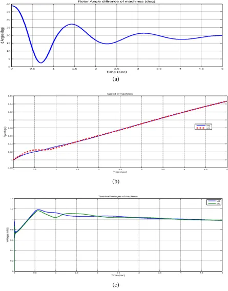
ESULTS

6.1.System analysis with-out FACTS

First trace on the Machines scope shows the rotor angle difference d_theta1_2 between the two machines. Power transfer is maximum when this angle reaches 90 degrees. It is a good signal for system stability. If d_theta1_2 exceeds 90 degrees for a long period of time, the machines

will be out of synchronism and the system becomes unstable. Machine speeds are represented by the second trace. It can be observed that machine 1 speed increases during the fault because during that period its mechanical power is higher than its electrical power. If the system is simulated for a long period of time (in seconds), it is also seen that the machine speeds oscillate together at a low frequency (Hz). The displayed waveforms are shown below. Here considering dynamic loading effect on bus-3

as shown in simulation fig. 5.

Pref1 Phasors powergui 2.968e+005 2.968e+005 1.954e+005 2.391e+005 V (VOLT S) B1 B2 B3 B4

m Pref

Pm Vf

T urbi ne & Regul ators M2

m Pref Pm Vf

abc Mag Pha

Sequence Anal yzer (Phasor T ype)2

abc Mag Pha

Sequence Anal yzer (Phasor T ype)

-C-Pref1

PSS PSS Bl ock

P Q2 P Q1

7.684e+008 1.274e+009 P Q (MW) B1

-5.454e+008 -3.426e+008 P Q (MW) B 3 1.546e+008

7.252e+008 P Q (MW) B 2 P Q Machi nes d_theta1_2 w1 w2 Vt1 Vt2 Machi ne Si gnal s

L3 150KM L2-2 150KM L2-1 150KM L1 280KM Vabc_B1 Iabc_B1 Vabc_B2 Iabc_B2 m A B C Dynamic Load A B C a b c B4 A B C a b c B3 A B C a b c B2 A B C a b c B1

A B C

50MW

Vabc Iabc

PQ

3-Phase Acti ve & Reacti ve Power

(Phasor T ype)3

Vabc Iabc

PQ

(Phasor T ype)

A B C

250MW A B C a b c 2100MVA 11KV/400KV Pm Vf _ m A B C 2100 MVA M1 A B C a b c 1400MVA 11KV/400KV Pm Vf _ m A B C 1400 MVA M2

A B C

100MW

(5)

The simulation results for test system with-out FACT are given below. The data for different parameters are given in

table 1.

0 0.5 1 1.5 2 2.5 3 3.5 4 4.5 5

0 5 10 15 20 25 30 35 40

Time (sec)

d

An

gl

e

(d

eg

)

Rotor Angle diffrence of machines (deg)

(a)

0 0.5 1 1.5 2 2.5 3 3.5 4 4.5 5

0.98 1 1.02 1.04 1.06 1.08 1.1 1.12 1.14 1.16

Speed of machines

Time (sec)

S

pe

ed

(p

u) M1M2

(b)

0 0.5 1 1.5 2 2.5 3 3.5 4 4.5 5

0 0.2 0.4 0.6 0.8 1 1.2 1.4

Time (sec)

V

ol

ta

ge

s

(vo

lts)

Terminal Voltages of machines

Vt1 Vt2

(6)

Fig.6 Waveforms for characteristics of machine (a) Rotor angle difference, (b) Speed of machines, (c) Terminal voltages of machines.

0 0.5 1 1.5 2 2.5 3 3.5 4 4.5 5

0 2 4 6 8 10

12x 10

5

Time (sec)

V

ol

ta

ge

s

(vo

lts)

Voltages at busB1,B2,B3,B4

V B1

V B2 (VB1=VB2) V B3

VB4

(a)

0 0.5 1 1.5 2 2.5 3 3.5 4 4.5 5

-2 -1.5 -1 -0.5 0 0.5

1x 10

9

Time (sec)

A

ct

ive

p

ow

er

P

(W

)

Active power at buses B1,B2,B3,B4

B1 B2 B3 B4

(b)

-0.5 0 0.5 1 1.5 2 2.5 3 3.5x 10

9

R

ea

ct

ive

p

ow

er

Q

(V

ar

)

Reactive power at buses B1,B2,B3,B4

(7)

Table-1 Active, Reactive power & voltages with-out FACTS

Bus

P (MW)

Q (Mvar)

S (MVA)

V (kv)

B1

768.4 1274

1487.79

296.8 B2

154.6

725.2

741.496

296.8 B3

-545.4

-342.6

664.08

195.4 B4

530.8

304.4

611.89

239.1

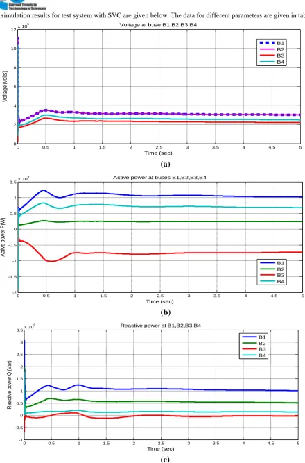
6.2 Impact of SVC

Here observe the impact of the SVC for stabilizing the network during a severe contingency. First put the two PSS in service. Verify that the SVC is in fixed susceptance mode with Bref = 0. The rating of the SVC is +/-1000 MVA, Start the simulation. In order not to pursue unnecessary simulation, the Simulink Stop block is used to stop the simulation when the angle difference reaches 3*360 degrees. Now open the SVC block menu and change the SVC mode of operation to Voltage regulation. The SVC will now try to support the voltage

by injecting reactive power on the line when the voltage is lower than the reference voltage (1.0 pu). The selected SVC reference voltage corresponds to the bus voltage with the SVC out of service. In steady state the SVC will

therefore be floating and waiting for voltage

compensation when voltage departs from its reference set point. Let we installed SVC at bus 3, because the voltage

at bus-3 is lower as seen with-out FACT analysis.

Pref1

Phasors

powergui

V (VOLT S) B1 B2 B3 B4

V

m Pref

Pm Vf

m Pref Pm Vf

m

A B C

SVC

abc Mag Pha

Sequence Anal yzer (Phasor T ype)

SVC

-C-Pref1

PSS PSS Bl ock

P Q3

P Q2 P Q1

P Q (MW) B1

P Q (MW) B 4 P Q (MW) B 3 P Q (MW) B 2

P Q Machi nes d_theta1_2 w1 w2 Vt1 Vt2 Machi ne Si gnal s

L3 150KM L2-2 150KM L2-1 150KM L1 280KM Iabc_B4 Vabc_B1 Iabc_B1 Vabc_B3 Vabc_B2 Iabc_B3 Vabc_B4 Iabc_B2 m A B C Dynamic Load A B C a b c B4 A B C a b c B3 A B C a b c B2 A B C a b c B1

A B C

50MW

Vabc Iabc

PQ

(Phasor T ype)4

Vabc Iabc

PQ

(Phasor T ype)3

Vabc Iabc PQ

(Phasor T ype)1

Vabc Iabc

PQ

(Phasor T ype)

A B C

250MW A B C a b c 2100MVA 11KV/400KV Pm Vf _ m A B C 2100 MVA M1 A B C a b c 1400MVA 11KV/400KV Pm Vf _ m A B C 1400 MVA M2

A B C

100MW

d_theta1_2 (deg) w1 w2 (pu) Vt1 Vt2 (pu) Vt1 Vt2 (pu)

(8)

The simulation results for test system with SVC are given below. The data for different parameters are given in table 2.

0 0.5 1 1.5 2 2.5 3 3.5 4 4.5 5

0 2 4 6 8 10 12x 10

5

Time (sec)

V

ol

ta

ge

(vo

lts)

Voltage at buse B1,B2,B3,B4

B1 B2 B3 B4

(a)

0 0.5 1 1.5 2 2.5 3 3.5 4 4.5 5

-2 -1.5 -1 -0.5 0 0.5 1 1.5x 10

9

Time (sec)

A

ct

ive

p

ow

er

P

(W

)

Active power at buses B1,B2,B3,B4

B1 B2 B3 B4

(b)

0 0.5 1 1.5 2 2.5 3 3.5x 10

9

R

ea

ct

ive

p

ow

er

Q

(V

ar

)

Reactive power at B1,B2,B3,B4

(9)

Bus P (MW) Q (Mvar) S (MVA) V (k volts) SVC data

V (pu) Q (pu)

B1 1028 1010 1441.14 301.5 - -

B2 243 518.7 572.799 301.5 - -

B3 -723.7 -37.3 724.66 221.8 0.6792 0.2416

B4 685.8 137.2 699.39 249.5 - -

7. C

ONCLUSION

This paper deals with applications of the SVC. The detailed models of the SVC is implemented and tested in MATLAB/simulink environment. The models are applicable for voltage stability analysis, and cover broader range of power transfer capability.

The effects of FACTS (SVC) installed in power transmission path are analyzed in this thesis, and the conclusions are as follow:

(1) The FACTS can improve voltage stability limit observably, and FACTS give better performance for power transfer capability for 4-bus system transmission capacity increased 67.27 MVA (SVC).

(2) The power losses in system with-out FACT is more as compared when used FACTS devices. The loading capacity with SVC is increased, the reactive power compensated form -342.6 MVAR (no FACTS) to -37.3 MVAR (SVC), and voltage injected from 195.4(no FACTS) to 221.8 kv (SVC), at bus-3 for 4-bus system. (3) The STATCOM give superior performance than SVC for reactive power, voltages and power transfer capability for both 4-bus and 6-bus system.

(4) Similarly the performance enhancement of 6-bus test system can be analyses for compensate reactive power, voltage injected and increased power transfer capability. (5) As has been discussed above (1)-(4) it has been observed system performance improved by introducing the FACTS Devices, the best performance has been obtained by introducing FACTS devices such as SVC which compensate reactive power (MVAR), voltage injected (kv) and increased power transfer capability (MVA). It‟s concluded that by introducing FACTS device system performance, voltage stability and transmission capability improves considerably.

R

EFERENCE

[2] Ding Lijie, Liu Yang, Miao Yiqun „Comparison of

grid‟ 978-0-7695-4077-1/10, 2010 IEEE, DOI 10.1109/ICICTA, 2010.

[3] Nimit Boonpirom, Kitti Paitoonwattanakij, „Static Voltage Stability Enhancement using FACTS‟ IEEE/PES

[4] Transmission and distribution Conference and Exhibition Asia Pacific., pp.1– 5, 2007.

[5] O. L. Bekri , M.K. Fellah, „Optimal Location of SVC and TCSC for Voltage Stability Enhancement‟ IEEE, 4th International Power Engineering and Optimization Conference (PEOCO 2010), Shah Alam, Selangor, MALAYSIA. 23-24 June 2010.

[6] H. Saadat, „Power System Analysis‟ McGraw-Hill

International Editions, 1999.

[7] V. K.Chandrakar, A.G.Kothari, „Optimal Location for LineCompensation by Shunt Connected FACTS Controller‟ 0-7803-788S-7/03/17.000 2003 IEEE.

[8] M.Kowsalya, K.K.Ray, and D.P.Kothari,

„Positioning of SVC and STATCOM in a Long Transmission Line‟ International Journal of Recent Trends in Engineering, Vol 2, No. 5, November 2009.

[9] Akhilesh A. Nimje, Chinmoy Kumar Panigrahi

and Ajaya Kumar Mohanty, „Enhanced power transfer capability by using SSSC‟ Journal of Mechanical Engineering Research Vol. 3 (2), pp. 48-56, February 2011.

[10] Dapu Zhao, Yixin Ni, Jin Zhong, Shousun Chen, „Reactive Power and Voltage Control in

Deregulated Environment‟ IEEE/PES

Transmission and Distribution Conference & Exhibition: Asia and Pacific Dalian, China, 2005. [12] George Gross, Paolo Marannino and Gianfranco

Chicco, „Reactive Support and Voltage Control Service: Key Issues and Challenges‟ IEEE MELECON 2006, May 16-19, Benalmadena (Malaga), Spain.

(10)

[14] J. J. Paserba, 'How FACTS controllers benefit AC transmission systems', in Proc. IEE Power Engineering Society General Meeting, Colorado, USA, 6-10 June, 2004, Vol. 2 (IEEE, Piscataway, NJ, 2004), pp. 1257-1262.

[15] Panda and R.N Patel, Transient Stability Improvement by Optimally Located STATCOMs Employing Genetic Algorithm', Intl J. Energy Technology and Policy, 5(4) (2007), 404-421. [16] R.Patel and K.V.Pagalthivarthi, 'MATLAB-Based

modelling of power system components in transient stability analysis', Intl J.Modelling and Simulation, 25(1) (2005), 43-50.

[17] P. Kundur, J. Paserba, V. Ajjarapu, G. Andersson, A. Bose, C. Canizares, N. Hatziargyriou, D. Hill, A. Stankovic, C. Taylor, T. V. Cutsem and V. Vittal, 'Definition and classification of power system stability', IEEE Trans. Power Systems, 19(2) (2004), 1387-1401.

[18] L. Gyugyi, 'Power electronics in electric utilities: static VAr compensators', IEEE Proc., 76 (1988), 483-494.

[19] L.Gyugyi, 'Dynamic compensation of a.c.

transmission lines by solid-state synchronous voltage sources', IEEE Trans. Power Delivery, 9(2) (1994), 904-911.

[20] B. T. Ooi, M. Kazerani, R. Marceau, Z. Wolanski, F. D. Galiana, D. Mcgills and G. Joos, 'Mid-point siting of FACTS devices in transmission lines', IEEE Trans. Power Delivery, l12 (1997), 1717- 1722.

[21] M.H.Haque,'Optimal location of shunt FACTS devices in long transmission lines', IEE Proc. Power Gen. Trans. Distrib., 147 (2000), 218-222. [22] S. Panda and R. N. Patel, 'Optimal location of

shunt FACTScontrollers or transient stability improvement employing genetic algorithms', Electric Power Components and Systems, 35(2) (2007), 189-203.

[23] M.H.Haque, 'Effects of exact line model and shunt FACTS devices on first swing stability limit', Intl J. Power Energy System, 25 (2005), 121-127. [24] N.G.Hingorani and L.Gyugyi, Understanding

FACTS Concepts and Technology of Flexible AC Transmission System (IEEE Press, New York, NY, 2000).

[25] R. M. Mathur and R. K. Varma, Thyristor-based FACTS Controllers for Electrical Transmission Systems (IEEE, Piscataway, NJ, 2002).

[26] Y. H. Song, Flexible AC Transmission Systems (FACTS) (IEE Press, London, 1999).

[27] G. Sybille and P. Giroux, 'Simulation of FACTS

[28] K.RPadiyar, “FACTS controllers in power

transmission and distribution” New Age

International Publishers.

[29] SimPowerSystemsUser guide.Available at

http://www.mathworks.com,

http//www.ieeexplore.com, www.google.com, etc.

[30] www.ijeetc.com/ijeetcadmin/upload/

IJEETC_50eabe01533c

[31] www.ukessays.com › Essays › Engineering [32] www.ieeexplore.ieee.org › ... › EmergingTrends in

Electrical

[33] www.journals.tubitak.gov.tr/elektrik/issues/elk-07-15.../elk-15-3-1-0601-5.pdf

[34] www.iosrjournals.org/ccount/click.php?id=2797