SURFACE ROUGHNESS
OPTIMIZATION BY RESPOSE
SURFACE METHODOLOGY AND
PARTICLE SWARM OPTIMIZATION
MEENU
Department of Mechanical Engineering, NIT, Kurukshetra, Haryana, 136119, India
[email protected] ANUJ KUMAR SEHGAL
Department of Mechanical Engineering, NIT, Kurukshetra, Haryana, 136119, India
[email protected] Abstract
Purpose: Manufacturability is an attribute which indicates how economically a component can be machined to
meet the specified requirements. This concept embraces the traditional indicators of machinability from the customer and manufacturer’s perspective. In this paper, Particle Swarm Optimization (PSO), an evolutionary technique is used to optimize the machining parameters in CNC end milling of Ferritic-Pearlitic Ductile Iron Grade 80-55-06 with the objective of minimizing the surface roughness.
Design/Methodology: Taking into account the parametric effect of spindle speed, feed rate and depth of cut,
central composite design (CCD) is employed in developing an efficient second-order response surface mathematical model. Analysis of variance (ANOVA) is used to test the adequacy of the developed mathematical model. Two methods, response surface methodology (RSM) and the Particle Swarm Optimization (PSO) are used to optimize the machining parameter i.e. surface roughness.
Findings: The solutions provided by the RSM for the best desirability value may further be confirmed in
conjunction with PSO to find the optimal solution and experimental settings.
Practical implications: The results showed that the PSO in confirmation with the response surface methodology
provides the high accuracy of results. The suggested PSO resulted to be an efficient and robust technique in machining processes. It has been found that the predicted surface roughness using PSO is in good agreement with the actual experimental value.
Originality/Value: The validation with 0.007 %ge is reported after the implementation of the findings by PSO
and suggested that the integrated approach of RSM and PSO to be an effective method for solving surface roughness optimization problems.
Keywords: Surface roughness, Metal, CNC milling, Central composite design (CCD), Response Surface Methodology (RSM), Analysis of Variance (ANOVA). Particle Swarm Optimization (PSO)
1. Introduction
speed and feed rates. The results were compared with other evolutionary techniques such as GA and SA and proved that the proposed technique improved the quality of the solution while speeding up the convergence process. A new technique has been proposed by Huang et al. [15] by using the combination of wavelet neural network (WNN) algorithm and modified PSO for solving tool wear detection and estimation. By using the Daubechies-wavelet, the cutting power signal is decomposed into approximation and details. The energy and square-error of the signals in the detail levels is used as characters which indicating tool wear, the characters are input to the trained WNN to estimate the tool wear. The results of the experiments were compared with BP neutral network, conventional WNN and GA-based WNN. The results showed a faster convergence and more accurate estimation of tool wear. The process parameters of milling operation such as spindle speed and feed rate were considered to be optimized in the study of Li et al. [16]. The considered machining performances were cutting force, tool-life, surface roughness and cutting power. An algorithm for process parameters optimization known as cutting parameters optimization (CPO) was introduced and PSO technique was employed to optimize the process parameters. From the experimental results, the authors concluded that PSO in optimizing process parameters can converge quickly to a consistent combination of spindle speed and feed rate. Chen et al. [17] proposed an improved PSO with opposition mutation (OMPSO) to select satisfied process parameter (depth of cut, feed rate, grit size) of grinding process. According to the researcher, OMPSO has the same tuning parameters as PSO and easy to use. The experiment result was compared to other evolutionary techniques such as GA, PSO and landscape adaptive PSO (LAPSO). It was obtained that the proposed technique was effective to solve grinding process optimization problem. In the research by Prakasvudhisarn et al. [18], process parameters of CNC end milling were selected such as feed rate, spindle speed, and depth of cut to find the minimum surface roughness. Support vector machine (SVM) was proposed to capture characteristics of roughness and its factors. PSO technique is then employed to find the combination of optimal process parameters. The results showed that co-operation between both techniques can achieve the desired surface roughness and also maximize productivity simultaneously. J.G. Li1 et al. [19], used particle swarm optimization (PSO) for cutting parameters optimization (CPO). The fundamental principle of PSO was introduced; then, the algorithm for PSO application in cutting parameters optimization was developed; thirdly, cutting experiments without and with optimized cutting parameters were conducted to demonstrate the effectiveness of optimization, respectively. The results showed the improvement in machining process.
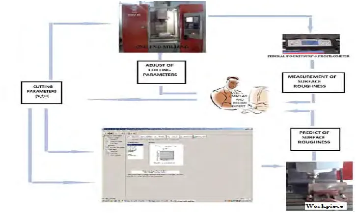
In this work, the Central composite design (CCD) under Response surface methodology is employed as Design of experiment for conducting the database in an end milling machining of Ductile Iron Grade 80-55-06. Analysis of variance (ANOVA) is used to test the adequacy of the developed mathematical model. Particle Swarm Optimization (PSO) is used to optimize the machining parameters and the same were compared with the experimental values. The research may be summarized by its purpose, as illustrated below in Fig.1.
2. Experimental Description
2.1 Selection of Experimental Design for Fitting Response Surface (Second Order Model)
The important aspect of response surface methodology is the design of experiments abbreviated as DoE. These strategies were originally developed for the model fitting of physical experiments, but can also be applied to numerical experiments. The objective of DoE is the selection of the points where the response should be evaluated. Most of the criteria for optimal design of experiments are associated with the mathematical model of the process. Generally, these mathematical models are polynomials with an unknown structure, so the corresponding experiments are designed only for every particular problem. The choices of the design of experiments can have a large influence on the accuracy of the approximation and the cost of constructing the response surface. Central composite design, the most popular class of design for fitting a second order model for surface Roughness (Ra) is used for this study. The experiments are conducted based on the central composite design (Fig. 2). The central composite design, introduced by Box and Wilson, contains imbedded factorial points (from a 2qfactorial design to 2(q k)fractional factorial design), central points and axial points. The number
of center points nc at the origin and the distance of the axial rums from the design center are two parameters in
Fig.1: Experimental Set-up
2.2 Materials, Machine Set-up, Test Conditions and Measurements
The factors whose effects are studied on the quality characteristics surface roughness in CNC milling are spindle speed (rpm), feed rate (mm/min.) and depth of cut (mm) on the quality characteristic surface roughness (Ra) in CNC end milling operation. The cutting process parameters and their levels selected are as shown in Table I. The set up employed a VMC (Vertical Milling Centre), two 4-flutes, and 10 mm diameter SGS-48554 cemented carbide end mill cutters. The machining was performed in dry environment and the Ra value of the machined workpiece was measured using the Federal Pocketsurf-3 Profilometer (Table II). The dimension of work material is taken as 80 mm x 75 mm x 15 mm. The specification of the work material is shown in Table III. The machining on specimen was made as per 20 different factor level combinations as representing the conduction of 20 experiments in Table IV. Before conducting the measurement, the instrument was calibrated using a standard roughness specimen to ensure the consistency and accuracy of Ra values. Five measurements were conducted along the length of cut on each workpiece and the average Ra value is recorded.
Table I: Cutting Process Parameters and Their Levels
Process Parameters (units)
Levels
-1.5 -1.0 0 1.0 1.5
Spindle Speed
(rpm) 1350 1500 1800 2100 2250
Feed Rate
(mm/min.) 12.5 15 20 25 27.5
Depth of Cut
(mm) 0.075 0.1 0.15 0.2 0.225
Table II: Experimental Setup And Conditions
Particulars Experimental conditions
Machine
Tool
Collet
Cutting parameters
Surface roughness tester
Coolant
Agni BMV- 45
MODEL No. BMV- 45, 12 stations automatic tool changer.
4 flute, 10.0 mm diameter, SGS 48554,Cemented carbide end mill cutter,
Size 8-10 mm
Depth of Cut, Cutting Speed, Feed Rate
Profilometer, Federal Pocketsurf-3, Piezoelectric contact type stylus, stylus travel: 0.1 inch/2.54 mm, maximum stylus force: 15 MN, measuring capacity: Ra or Rmax/Ry or Rz
Table III: Specification Of Work Material
Particulars Value
Material Ductile Iron Grade 80-55-06
Minimum Tensile Strength 80 psi (552 MPa)
Yield Strength 55 psi (379 MPa)
% Elongation 6%
Typical Brinell Hardness 200 BHN
Matrix-microstructure Pearlite and Ferrite
Fig. 2: Central Composite Design
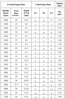
Table IV: Process Parameters & Their Levels
Uncoded Input Data Coded input Data Output
Data
Spindle Speed (rpm)
Feed Rate (mm/min.)
Depth of Cut
(mm)
X1 X2 X3 Ra
(µm)
1800 20 0.15 0 0 0 1.74 1500 25 0.2 -1 1 1 4.45
1500 25 0.1 -1 1 -1 3.79
1800 20 0.15 0 0 0 1.64
2100 15 0.1 1 -1 -1 1.58
2100 25 0.2 1 1 1 3.69
2100 15 0.2 1 -1 1 1.78
1800 20 0.15 0 0 0 1.84
1500 15 0.1 -1 -1 -1 2.39 1500 15 0.2 -1 -1 1 1.6
1800 20 0.15 0 0 0 1.62
2100 25 0.1 1 1 -1 3.62
1800 20 0.15 0 0 0 1.98
1800 12.5 0.15 0 -1.5 0 1.38
1800 20 0.15 0 0 0 1.77
1800 20 0.075 0 0 -1.5 1.81
1800 27.5 0.15 0 1.5 0 4.52
1800 20 0.225 0 0 1.5 2.29
2250 20 0.15 1.5 0 0 2.12
3.DEVELOPMENT OF MATHEMATICAL MODEL AND PREDICTION OF SURFACE ROUGHNESS BY RESPONSE SURFACE METHODOLOGY
Response surface method is a collection of mathematical and statistical technique, useful for the model and analysis of problems in which a response of interest is influenced by several variables. The methodology is used for determining and representing the cause-effect relationship between the response and the input control variables as a two or three dimensional hyper surface. The considerable success of response surface
methodology in manufacturing industries under various situations is evident [3, 4], thus in the present work an empirical relation is developed in order to-relate the surface roughness as a function of various machining parameters. In many engineering fields with the aid of experimental conditions, it is possible to represent the relationship between the response ‘y’ and set of controllable variables
x1, x2xn
. Then, a model can bewritten in the form
yf ( x x1, 2,xn) (1)
Where ε represents error observed in the response ‘y’and the function ‘f’ is called response surface or response function. If the expected response is denoted by E(y) then the expected response surface may be represented as,
E(y)f ( ,x x1 2,xn) (2)
Usually the best suited second order model is utilized in the response surface methodology when response is a function of more than one variable.
2 0
1 1
k k
y i ix ii ix ij i jx x
i j
i i
(3) The coefficient, in the second order model is obtained by the least square method. The observations of response (Surface Roughness) are illustrated in Table IV. The steps involved under the said methodology are adopted as under:(i) Identification of important process control variables.
(ii) Considering the appropriate upper and lower limits of the process control variables, i.e. spindle speed (s), feed rate (f) and depth of cut (d).
(iii) Conducting the experiments as per the selected central composite experimental design (Table IV) and recording of response (s) viz. surface roughness.
(iv) Development of second order quadratic model and determining coefficients of the second order polynomial. (v) The adequacy of developed model and testing the significance of regression coefficients.
(vi) Analyzing and presentation of main effects and significant interaction effects of process control parameters in term of contour plots and surface plots.
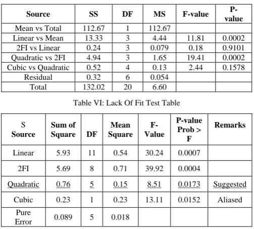
(vii) Determination of optimized machined process parameters for the response (surface roughness). Table V: Design Matrix Evaluation For Response Surface Quadratic Model
Source SS DF MS F-value
P-value
Mean vs Total 112.67 1 112.67
Linear vs Mean 13.33 3 4.44 11.81 0.0002 2FI vs Linear 0.24 3 0.079 0.18 0.9101 Quadratic vs 2FI 4.94 3 1.65 19.41 0.0002 Cubic vs Quadratic 0.52 4 0.13 2.44 0.1578
Residual 0.32 6 0.054
Total 132.02 20 6.60
Table VI: Lack Of Fit Test Table
S
Source
Sum of
Square DF
Mean Square
F- Value
P-value Prob >
F
Remarks
Linear 5.93 11 0.54 30.24 0.0007
2FI 5.69 8 0.71 39.92 0.0004
Quadratic 0.76 5 0.15 8.51 0.0173 Suggested
Cubic 0.23 1 0.23 13.11 0.0152 Aliased
Pure
The analysis is done using uncoded units. The employed Design Expert-7 software computed the linear, quadratic and interaction terms in the model. From Table V, the quadratic model is suggested with the p-value of 0.0002.Table VI shows the lack of fit test which assess the fit of the developed model and suggested the model to be quadratic. The adequacy of the model is tested at 95% confidence interval. The most useful technique in the field of statistical inference i.e. Analysis of Variance (ANOVA) is performed to justify the validating of the 2nd order model.
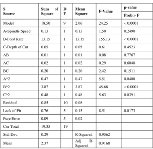
Table VII: ANOVA Table
S Source
Sum of Square
D F
Mean
Square F-Value
p-value
Prob > F
Model 18.50 9 2.06 24.25 < 0.0001
A-Spindle Speed 0.13 1 0.13 1.50 0.2490
B-Feed Rate 13.15 1 13.15 155.13 < 0.0001
C-Depth of Cut 0.05 1 0.05 0.61 0.4523
AB 0.01 1 0.01 0.08 0.7767
AC 0.02 1 0.02 0.29 0.6048
BC 0.20 1 0.20 2.42 0.1511
A^2 0.47 1 0.47 5.51 0.0408
B^2 3.87 1 3.87 45.68 < 0.0001
C^2 0.48 1 0.48 5.63 0.0391
Residual 0.85 10 0.08
Lack of Fit 0.76 5 0.15 8.51 0.0173
Pure Error 0.09 5 0.02
Cor Total 19.35 19
Std. Dev. 0.29 R-Squared 0.9562
Mean 2.37 Adj
R-Squared 0.9168
The ANOVA consists of degree of freedom (D.F.) and sum of square (SS). The sum of sequence is usually contributed from the regression model and residual error. Mean square (MS) is the rate of mean square to the degree of freedom (DF). F- Ratio is the rate of mean square of regression model to the mean square of residual error. From the ANOVA table, the small P values for model, linear and square terms point out that their contribution is significant to the model. Moreover, the main effects other than depth of cut can be referred to be significant as per Table VII. The quadratic terms A2, B2, C2 and interaction term BC significantly contribute to the response model at 95 % confidence level, thus the final model correlating surface roughness (Ra) with cutting parameters is found as follows:
R 19.63- 0.009 - 0.84 - 43.93 - 0.00002 .v f d v f 0.0037 .v d 0.64 .f d 0.00000237v2 0.025f2 86.1d2
a
(4)
Here process control variables are uncoded values. Further, from Table VII, it is evident that the model is adequate at 95% confidence level. Among the factors considered feed rate is found to be the most significant parameter. The effectiveness of the model is checked by using the ‘R2’ value i.e. 0.96 which is very close to 1 and hence the model is found to be very effective. The validity of the model is reconsidered with the adjusted correlation coefficient i.e. ‘R2(adj)’value = 0.92, which is a measure of the variability of the observed output and can be explained by the factors along their factor interactions.
confidence interval includes 1, indicating no transformation is recommended. The correlation scatter graph as shown in Fig. 7, suggest the very good agreement between the experimental values and the predicted values obtained by the mathematical model.
Design-Expert® Sof tware Surf ace Roughness
Lambda
Current = 1
Best = 0.24 Low C.I. = -1.9 High C.I. = 2.03
Recommend transf orm: None (Lambda = 1)
X: Lambda Y: Ln(ResidualSS)
Box-Cox Plot for Power Transforms
-0.23 0.03 0.28 0.53 0.78
-3 -2 -1 0 1 2 3
Design-Expert® Sof tware Surf ace Roughness
Color points by v alue of Surf ace Roughness:
4.50
1.38
X: Actual Y: Predicted
Predicted vs. Actual
1.30 2.15 3.00 3.85 4.70
1.38 2.20 3.01 3.83 4.64
Fig. 4: Normal Probability plot Fig. 5: Plot of residuals vs Fig. 6: Box-Cox plot for Fig.7: Correlation graph of residuals for Ra data run numbers for Ra data power transforms
From the interaction surface plots, Fig. 8, illustrates the surface roughness by varying the two variables and keeping the third factor at optimum level as per the findings from ramp diagram. The figures indicate that surface roughness increases with the increase in feed rate, followed by spindle speed and among the interaction between variables; the AB variable pair interaction represents the greatest contribution. The developed models are used for the response optimizations by desirability function approach to obtain minimum surface roughness (Ra).
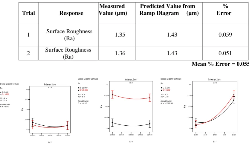
Table VIII: Confirmation Experiment For The Response Optimization
Trial Response
Measured Value (µm)
Predicted Value from Ramp Diagram (µm)
% Error
1 Surface Roughness
(Ra) 1.35 1.43 0.059
2 Surface Roughness
(Ra) 1.36 1.43 0.051
Mean % Error = 0.055
Design-Expert® Sof tware
Ra
C- 0.100 C+ 0.200
X1 = A: v X2 = C: d
Actual Factor B: f = 16.42
C: d
1500.00 1650.00 1800.00 1950.00 2100.00
Interaction A: v Ra 1.3 2.125 2.95 3.775 4.6
Design-Expert® Sof tware
Ra
B- 15.000 B+ 25.000
X1 = A: v X2 = B: f
Actual Factor C: d = 0.17
B: f
1500.00 1650.00 1800.00 1950.00 2100.00
Interaction A: v Ra 1.1 1.975 2.85 3.725 4.6
Design-Expert® Sof tware
Ra
C- 0.100 C+ 0.200
X1 = B: f X2 = C: d
Actual Factor A: v = 1789.43
C: d
15.00 17.50 20.00 22.50 25.00
Interaction B: f Ra 1.1 1.975 2.85 3.725 4.6
Fig.8 Interaction effects of factors.
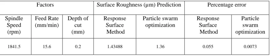
v = 1841.50
1500.00 2100.00
f = 15.60
15.00 25.00
d = 0.20
0.10 0.20
Ra = 1.43488 1.42
2
1.38 4.52
Desirability = 0.974
Fig. 9: Ramp diagram with optimized machining parameters and predicted response
4. Particle Swarm Optimization (PSO)
PSO technique was introduced in 1995 by Kennedy and Eberhart [ 20] and an evolutionary technique in solving continuous optimization problems [21]. The swarm is composed of volume-less particles with stochastic velocities, each of which represents a feasible solution. The algorithm finds the optimal solution through moving the particles in the solution space. PSO is a very simple concept, and paradigms are implemented in a few lines of computer code. It requires only primitive mathematical operators, so is computationally in expensive in terms of both memory requirements and speed.
4.1. PSO methodology
The implementation of PSO is very simple and needs only a few lines programming code. It requires uncomplicated mathematical operators; therefore it is computationally economical in terms of both memory requirements and speed. PSO has features of both GA and evolution strategies. The PSO considers a swarm S
containing n particles (S = 1,2 ...n) in a d-dimensional continuous solution space. The position and velocity of individual i are represented as the vectors xi = (xi1………xid) and vi = (vil………..vid), respectively. A bird adjusts its position in order to find a better position, according to its own experience and the experience of its companions. Using the information, the updated velocity of individual i is modified using equation 5.
(5)
where t id
v = Component in dimension d of the ith particle velocity in iteration t
t id
x = Component in dimension d of the ith particle position in iteration t
1
c , c2 = weight factors
i
p = Best position achieved so long by particle i
g
p = Best position achieved so long by neighbours of particle i
1 2,
r r are random factors in range [0,1]
w = inertia weight
The steps of optimizing process parameters of milling operation using PSO as per [14] is as follows.
(i) Generation and initialization of an array of n particles with random positions and velocities. Velocity vector has three dimensions, feed rate and spindle speed and depth of cut.
(ii) Evaluation of objective function (surface roughness) for each particle. (iii) Obtain the pbest (personal best) of each particle and gbest (global best) (iv) Update the velocity and position.
(v) The objective function values are calculated for new positions of each particle. If a better position is achieved by particle, the pbest value is replaced by the current value and the best value obtained so far by any particle in the neighborhood of that particle (gbest) is found
(vi) Steps (iv) and (v) are repeated until the iteration number reaches a predetermined iteration.
1
1 1* – 2 2* ( – )
t t t t t t
id id id id gd id
4. 2 Control parameters of PSO
The effect of machining parameters on the surface roughness was studied. In present optimization problem the particles in space is taken as 5. The fitness parameter considered as minimization of surface Roughness. The all particles are evaluated by the fitness parameter and have velocities for the particles. The optimization based on PSO was executed using MATLAB software with number of generations considered as 50. These particles are assumed to fly through the problem space by following the current optimum particles. The c1, c2 are the weight factors or learning factors and found to 0.8, 2 respectively. The inertia weight w is computed to be 0.9 which is closer to 1, represents the good control on the momentum of the particle. Table IX shows the control parameters of PSO in tabulated form.
Table IX: The control parameters of PSO
4.3 Result
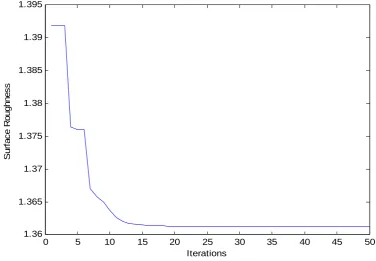
Experiments are performed on CNC end milling machine according to the Central composite design as shown in Table IV. The RSM methodology is adopted in order to predict the response with the selected combination of machining settings with the maximum desirability found to be 1.43 (µm). The evaluation of objective function (surface roughness) for each particle is programmed to obtain the pbest (personal best) of each particle and gbest (global best) by uupdating of the velocity and position in various iterations. Fig 10 shows how surface roughness decreases with number of iterations. The objective function values are calculated for new positions of each particle. If a better position is achieved by particle, the pbest value is replaced by the current value and the best value obtained so far by any particle in the neighborhood of that particle (gbest) is found. Fig 10 (surface roughness vs number of iterations) shows how surface roughness decreases with number of iterations. The predicted value of surface roughness is found to be 1.36 (µm)and the optimum process parameters are obtained to be spindle speed (1841.5 rpm), feed rate (15.6 mm/min.), depth of cut (0.2 mm). The confirmation experimental values are obtained and are used in conjunction with PSO as per Table VIII to obtain the mean error.
Hence, it can be concluded from the optimization results of the PSO program that it is possible to select a combination of feed rate, cutting speed and depth of cut to achieve the required surface roughness in machining process. The application of a PSO approach to obtain optimal machining conditions will be quite useful at the computer-aided process planning (CAPP) stage in the production of high-quality goods with tight tolerances by a variety of automated machining operations and in adaptive control machine tools. With the known boundaries of desired characteristic and relevant machining conditions, the machining can be performed with a relatively high rate of success with the selected machining conditions.
Table X. Comparison of the Output values of the surface roughness with respect to input machining parameters by RSM and PSO
Factors Surface Roughness (µm) Prediction Percentage error Spindle
Speed (rpm)
Feed Rate (mm/min)
Depth of cut (mm)
Response Surface Method
Particle swarm optimization
Response Surface Method
Particle swarm optimization
1841.5 15.6 0.2 1.43488 1.36 0.055 0.0073
PSO Parameters Value
Fitness parameter Minimization of surface Roughness
Number of generations 50
Number of particles 5
0 5 10 15 20 25 30 35 40 45 50 1.36
1.365 1.37 1.375 1.38 1.385 1.39 1.395
Iterations
S
ur
fac
e
R
ou
ghn
es
s
Fig 10. Surface Roughness vs Iterations 5. Conclusions
In the present study, surface roughness prediction model based on the two research approaches viz. design of experiment and Particle swarm optimization are attempted successfully. The performance of the developed model by both approaches is found to be reasonably good with percentage mean errors of 5.5% and 0.07% respectively. The response surface modeling has shown the feasibility of predicting optimum response easily and successfully at the factor level settings for the surface roughness value to be 1.43 µm with mean % error of 5.5% in comparison to confirmation experimental values. On the other hand the model prediction based on particle swarm optimization is found outperforming the RSM. The main advantages of the PSO algorithm are summarized as: simple concept, easy implementation, robustness to control parameters and computational efficiency when compared with mathematical algorithm and other heuristic optimization techniques thus may be extended to determine other parametric prediction for various machining conditions and processes for the other grades of ductile iron family.
REFERENCES
[1] http://www.ductile.org, Ductile iron society, 2012.
[2] Goodrich, G. M., 2007, Case histories of cast iron machinability problems, http://www.allbusiness.com/manufacturing/fabricated-metal-product-manufacturing/630735-1.html on line 08/08/2007
[3] Lela B, Bajic d, jozic S., 2008. Regression analysis, support vector machine and Bayesian neural network approaches to modeling surface roughness in face milling, Int J Adv manuf. Technolo. Doi: 10.1007/s00170-008-1678-z.
[4] Zhang J. Z., J.C. Chen, E.D. Kirby., 2007. Surface roughness optimization in an end-milling operation using Taguchi design method, Journal of Materials Processing Technology, 184233-239.
[5] Benardos, P. G and Vosniakos, G.C., 2002.Prediction of surface roughness in CNC face milling using neural network and Taguchi’s design of experiment, Robotics and Computer Integrated Manufacturing, 18 (5-6), 343-354.
[6] Benardos, P. G and Vosniakos, G.C., 2003, Predicting surface roughness in machining: a review, International Journal of machine tools and Manufacture, 43 (8), 833-844.
[7] Abbasi B., M. Hashem., 2012. Improving response surface methodology by artificial neural network and simulated annealing., Journal of Expert Systems with Applications Vol.39, pp. 3461-3468.
[8] Salah Al-Zubaidi, Jaharah A. Ghani, and Che Hassan Che Haron,. 2011.Application of ANN in Milling Process: A Review, Journal of Modeling and Simulation in Engineering Volume 2011, Article ID 696275, pages-7.
[9] M. Adam Khan & A. Senthil Kumar & A. Poomari, 2011. A hybrid algorithm to optimize cutting parameter for machining GFRP composite using alumina cutting tools. Int J Adv Manuf Technol DOI 10.1007/s00170-011-3553-6.
[10] Bharathi, R. S., & Baskar, N. (2011). Particle swarm optimization technique for determining optimal machining parameters of different work piece materials in turning operation. International Journal of Advanced Manufacturing Technology, 54(5–8), 445–463. [11] Amir Mahyar Khorasani, M. R. S. Yazdi, M. , Safizadeh, 2011, “Tool Life Prediction in Face Milling Machining of 7075 Al by Using
Artificial Neural Networks (ANN) and Taguchi Design of Experiment (DOE)”, IACSIT International Journal of Engineering and Technology, Vol.3, No.1, pp. 30-35.
[12] Md. Anayet Ullah Patwari, A. K. M. Nurul Amin and Muammer D. Arif, 2011. Optimization of Surface Roughness in End Milling of Medium Carbon Steel by Coupled Statistical Approach with Genetic Algorithm, The First International Conference on Interdisciplinary Research and Development, Thailand 31 May - 1 June, 2011, pp. 41.1-41.5.
[14] Zu˘ perl, U., Cu˘ s, F., & Gecevska, V., 2007. Optimization of the characteristic parameters in milling using the PSO evolution Technique, Journal of Mechanical Engineering, vol. 6, pp.354–368.
[15] Huang, H., Li, A., & Lin, X. 2007. Application of PSO-based wavelet neural network in tool wear monitoring. Proceedings of the IEEE international conference on automation and logistics pp. 2813–2817.
[16] Li, J. G., Yao, Y. X., Gao, D., Liu, C. Q., & Yuan, Z. J. , 2008. Cutting parameters optimization by using particle swarm optimization (PSO). Applied Mechanics and Materials Vol.5, 10-12, 879–883.
[17] Chen, Z. & Li, Y., 2008. An improved particle swarm algorithm and its application in grinding process optimization, Proceedings of the 27th Chinese Control Conference, pp. 2–5.
[18] Prakasvudhisarn, C., Kunnapapdeelert, S., & Yenradee, P., 2009. Optimal cutting condition determination for desired surface roughness in end milling, International Journal of Advanced Manufacturing Technology, 41(5–6), 440–451.
[19] J.G. Li1, Y.X. Yao1, D. Gao1, C.Q. Liu1 and Z.J. Yuan, 2008. Cutting Parameters Optimization by Using Particle Swarm Optimization (PSO), Applied Mechanics and Materials Vols. 10-12 pp. 879-883
[20] Kennedy, J. & Eberhart, R. C., 1995. Particle swarm optimization, Proceedings on IEEE international conference on neural networks, IV, pp. 1942–1948.