Application of diffusion laws to composting: theory, implications, and experimental testing

(1)

APPLICATION OF DIFFUSION

LAWS TO COMPOSTING:

THEORY, IMPLICATIONS, AND

EXPERIMENTAL TESTING

A thesis

Submitted in partial fulfilment

of the requirements for the Degree of

Ph.D.

at

Lincoln University

by

P. D. Chapman

Lincoln University

(2)

Abstract

of a thesis submitted in partial fulfilment of the requirements for the degree of Ph.D.

APPLICATION OF DIFFUSION LAWS TO COMPOSTING:

THEORY, IMPLICATIONS, AND EXPERIMENTAL TESTING

by

P. D. Chapman

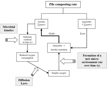
Understanding the fundamentals of composting science from a pragmatic perspective of necessity involves mixtures of different sizes and types of particles in constantly changing environmental conditions, in particular temperature. The complexity of composting is affected by this environmental variation. With so much „noise‟ in the system, a question arises as to the need to understand the detail of this complexity as understanding any part of composting with more precision than this level of noise is not likely to result in greater understanding of the system. Yet some compost piles generate offensive odours while others don‟t and science should be able to explain this difference. A driver for this research was greater understanding of potential odour, which is assumed to arise from the anaerobic core of a composting particle. It follows that the size of this anaerobic core could be used as an indicator of odour potential. A first step in this understanding is the need to determine which parts of a composting particle are aerobic, from which the anaerobic proportion can be determined by difference. To this end, this thesis uses a finite volume method of analysis to determine the distribution of oxygen at sub-particle scales. Diffusion laws were used to determine the thickness of each finite volume.

(3)

This first version of micro-environment analysis was derived from the simpler solution to diffusion laws, based on the assumption of non-diffusible substrate. It was tested against three sets of experimental data with two different substrates:

 Particle size trials using dog sausage as substrate – where the peak composting rate

was successfully predicted, as a function of particle size.

 Temperature trials using pig faeces and a range of particle sizes – The results

showed the potential of micro-environment analysis to identify intriguing

temperature effects, in particular, a different temperature effect (Q10) and fraction

proportion was indicated for each substrate fraction. Smaller particle sizes, and possibly outward diffusion of substrate confounded a clear experimental signal.

 Diffusion into a pile trials which showed that the time course of particles deeper in

the pile could be predicted by the physics of oxygen distribution. A fully computed prediction would need an added level of computational complexity in micro-environment analysis, arising from there being two intertwined phases, gas phase and substrate (particle) phase. Each phase needs its own

micro-environment calculations which can not be done in isolation from each other.

Unexplainable parts of the composting time course are likely to be partly explained by the outward diffusion of substrate towards the inward-moving oxygen front. Although the possibility of alternative electron acceptors can not be discounted as a partial explanation.

To test the theory, a new experimental reactor was developed using calorimetry. With an absolute sensitivity of 0.132 J hr-1 L-1 and a measurement frequency of 30 minutes, the reactor was able to detect the energy required to humidify the input air, and „see‟ when composting begins to decline as oxygen is consumed. Optimisation of the aeration pumping frequency using the evidence from the data was strikingly apparent immediately after setting the optimum frequency.

Micro-environment analysis provides a framework by which several physical effects can be incorporated into compost science.

(4)

List of Figures

Figure 1-1 – Compost knowledge with low precision measurement ability at sub-particle scales. 2 Figure 1-3 –Diagrammatic representation of the impact that the presence of oxygen has on the

utilization of nitrates as electron acceptor. 4

Figure 3-1 – The adjustment factor due to Monod kinetics (Equation 3-4; KO2 = 3.5 x 10-4 g O2 L-1). 22

Figure 3-2 - A typical composting profile, under assumed conditions. 31 Figure 3-3 – Oxygen concentration profiles with a 6-hour separation, assuming only the fast fraction is

composting. Data using Bouldin’s (1968) model II with k=10 W MJ-1 & E = 0.002 MJ cm-3. 32 Figure 3-4 – The influence of length of analysis interval on determination of the oxygen penetration

velocity (cm/day) of Figure 3-3. The 0.0087 cm/day velocity at the 6 hour interval in Figure 3-3.

reduces to 0.00825 cm/day as the interval → 0. 33

Figure 3-5 – The relative degradation rates of an aerobic fast fraction and the same fraction with an anaerobic rate constant assumed to be two orders of magnitude less than the aerobic rate

constant. 36

Figure 3-6 – Micro-environment state-space with a finite time interval. Where m denotes the

micro-environment index and ti is the time step. 38

Figure 3-7 - Diagrammatic representation of the nature of oxygen penetration into a composting

particle and the development of micro-environments. 41

Figure 3-8 - The effect of particle geometry on the proportion of the aerobic zone in the fuzzy layer

(composting rate < 50% of maximum - Equation 3-7). 45

Figure 3-9 – Diagram showing the mechanisms involved in the formation of a new micro-environment in a time interval (ti). Where: μenv = micro-environment. 46

Figure 4-1 – Space-time-particle size-substrate relationships between different micro-environments. Where the aerobic composting rates QA > QB > QC > QD. 51

Figure 4-2 - Discretising time into units, with a corresponding discretisation of the space dimension, representing the step-wise advance of the ‘aerobic front’ into a composting particle along dimension m (m will be a linear depth for a slab-shaped particle with planar geometry, or

inwards along the radius r for a spherical particle). 52

Figure 4-3 – The effect of changing (n) on Stępniewski’s multilayer model. Fast fraction rate constant only with a layer thickness zm of 0.001 cm; where



 

n m

m 1zm = depth as determined by Equation

4-9. Notes: 1) The VOR of each layer is the same – including the n+1 layer. 2) The n curve does not neatly meet the axis as the thickness of the layers (zm = zn = 0.001 cm), does not exactly

match the oxygen penetration depth (0.03023 cm). 59

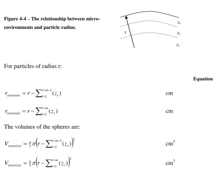
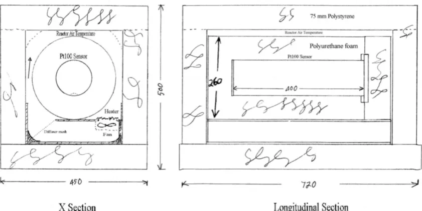
Figure 4-4 – The relationship between micro-environments and particle radius. 63 Figure 5-1 – The reactor with its coil. Air entered the bottom pipe and exited the top pipe on the RHS.

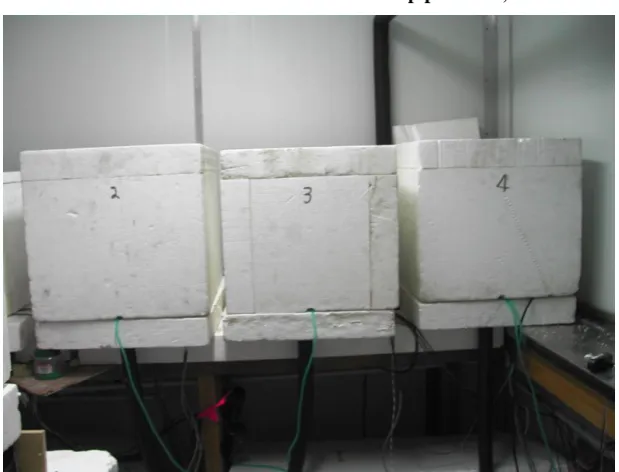
76 Figure 5-2 - The reactor in its insulation with sensors and air pipes fitted, located in its wooden box.

(10)

Figure 5-3 – The reactor assemblies in their polystyrene covers. The data loggers, power supply and control circuits were housed under the polystyrene cover at the base of the picture. Six reactors (one of which was the diffusion reactor) were housed in this cool room. 76 Figure 5-4 – Reactor sections. Showing sensor locations and reactor air circulation. The heaters

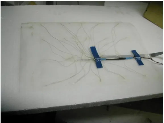
were electrical resistors located immediately above the fan. 78 Figure 5-5 – The thermocouple array which was folded around the sixth reactor used for diffusion

trials. Reference temperature for all thermocouples was the Pt100 sensor in the centre of the

array. 79

Figure 5-6 – Using reactor heat output time course (hours) to determine optimum aeration pumping

delay. 30 minute final storage frequency. 86

Figure 5-7 – Longitudinal temperature profiles along the reactor as influenced by the composting rate where day 1= maximum composting rate. Compost set temperature = 20 °C. Data from a thermocouple sensor array with 5 locations along the reactor and each location being an average

of 4 positions around the reactor (Figure 5-5). 89

Figure 5-8 – Average reactor temperature (average of 20 sensor locations along and around the reactor wall) expressed as the difference from the Pt100 sensor, and as a % of delta T across the

insulation. 89

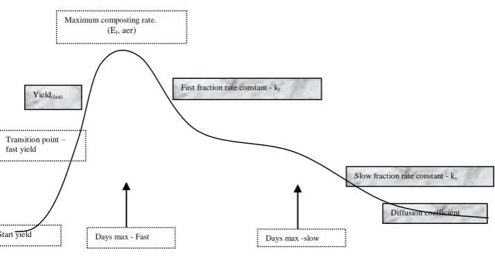
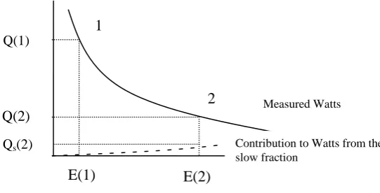
Figure 5-9 – Diagram showing aspects of the composting time course that can aid determination of parameters. Note: textured boxes refer to parameters which impact primarily the ‘slope’ of the data curve, while dotted boundaries indicate those parameters which are primarily positional – they change the position of the data curve. The interconnectedness of the parameters means that any categorisation as above will be an incomplete explanation of the composting time course.

94 Figure 5-10 – Points on the heat output versus energy remaining over time schematic, used for

determining fast fraction rate constant and fraction proportion. 95 Figure 5-11 – Points on the heat output versus energy remaining schematic, used for determining slow

(and subsequent) fraction rate constants and fraction proportions. 97 Figure 5-12 -Lineweaver Burke plot with three fractions. Data from faeces trial 1, 120C reactor. 102 Figure 5-13 – Four analysis intervals and their effect on the output of the MEA model using 1.33 cm

particle size of pig faeces at 200C. 103

Figure 6-1 – Measured versus modelled composting time course of the 0.8 cm cubical particle size; and

time course of the aerobic proportion. 105

Figure 6-2 - Measured versus modelled composting time course of the cubical particles of size 1 cm and 2.5 cm.5 Model used the same parameters as determined for the 0.8 cm cubical particle size (Figure 6-1). The micro-environment model was run with only particle size changed. 106 Figure 6-3 – Measured versus modelled composting time course of the cubical particles of size 1.5 cm

(11)

Figure 6-5 – The 1 cm dog sausage data with 2 theoretical perspectives on the fast fraction: Micro-environment analysis with only an exponential growth phase parameter; micro-Micro-environment analysis with both exponential + logarithmic growth phase parameters. 110 Figure 6-6 – Dog sausage oxygen penetration distance over time, calculated with the MEA model.

Minimum depth occurs at fast fraction maximum composting rate (day 2). The end of the growth phase (fast & slow) is day 13. Up to this point, periods where z may be negative (e.g. the flat section at day 8), caused problems with the formal structures of micro-environment analysis.

113 Figure 6-7 – Modelled versus measured composting rate for 1.33 cm pig faeces particles with 2

diffusion coefficients. Note the lower diffusion coefficient required more substrate (0.015 v 0.01

MJ cm-3) for the model to fit the data curve. 115

Figure 6-8 - Dog sausage trial 2, the 2.5 cm cubical particles composting rate expressed as a surface oxygen flux, compared with the output of Equation 6-7, where VOR is determined by the MEA

model. 118

Figure 6-9 - Faeces trial 2. Composting rates for three (6, 12, 20 0C) of the 5 reactors. 121 Figure 6-10 – Composting rates for three particle sizes from the pig faeces trial, modelled using MEA

with parameters determined from the 1.33 cm particle. The mass fraction of the faeces in the 1.8 cm size was 0.312; 1.33 cm was 0.23; 0.8 cm was 0.194; the remainder was <0.8 cm in size and had a faeces mass fraction of 0.035. The remaining proportion 0.229 was BM. 123 Figure 6-11 -The time course of the aerobic proportion for the 3 particle sizes in Figure 6-10, from the

MEA model. 124

Figure 6-12 – Fast fraction rate constants determined for pig faeces in trial 2 as compared with an Arrhenius adjustment (Q10 = 2) and an adjustment of 1.49. Rate constants were determined

with both first-order kinetics and a micro-environment model run without adjusting for

solubility in water and diffusion coefficient. 128

Figure 6-13 Slow fraction rate constants for pig faeces in trial 2, as compared with an Arrhenius adjustment (Q10 = 2) and an adjustment of 1.49. Rate constants were determined with both

first-order kinetics and a micro-environment model run without adjusting for solubility in water

and diffusion coefficient. 128

Figure 6-14 Results from pig faeces temperature trial 2 showing the experimentally determined days to maximum composting rate for both fast and slow fractions. The Arrhenius relationship (with a Q10=2) is also shown, plus polynomial curves fitted to the measured data. 132

Figure 6-15 Pig faeces trial 2, 20 0C reactor with fitted curve using 3 factions and first-order kinetics. 133 Figure 6-16 – The modelled time course of energy production of dog sausage 1 cm cubical particle with

three different interstitial oxygen concentrations (mg L-1). 135 Figure 6-17 - Temperature difference from the average (0C), of 5 sensors evenly spaced down 400 mm

(12)

Figure 7-1- Oxygen consumption rate of chicken manure from Hamelers (2001) 2mm diameter particle data (extracted from graph A, Figure 7-2), analysed with the MEA model for his other particle sizes. MEA modelled data assumes no diffusion of substrate. 148 Figure 7-2 - Hamelers (2001 p.181). Composting time course for chicken manure with A) 2mm, B)

(13)

List of Tables

Table 0-1 – Parameters and their relationship to scale. ... xvii

Table 0-2 – The relationship between micro-environment time and pile composting time. ... xviii

Table 3-1 –Estimated interval giving a 2% reduction (E/E0 = 0.98) in the composting rate using Equation 3-13 and 1 order of magnitude between the rate constant of each fraction (kf = 10; ks = 1; kh = 0.1 W MJ-1). ... 26

Table 3-2 – Possible phenomenological rate constants from three substrates and three electron acceptors. ... 30

Table 5-1 – Thermal conductivity as influenced by moisture content. ... 84

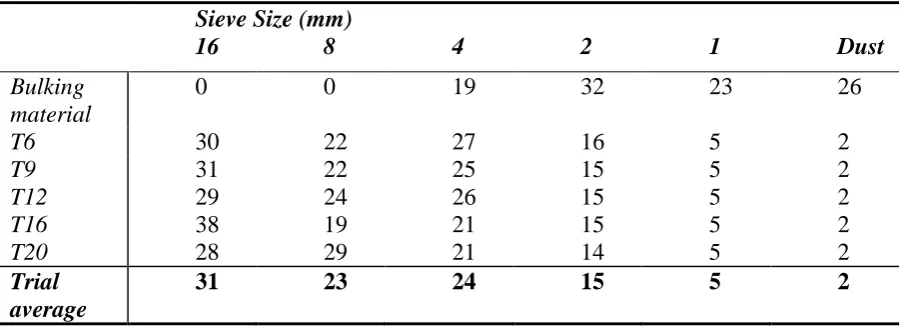
Table 5-2 – The equivalent spherical diameter and FAS of the cubical particles. ... 92

Table 5-3 The % of oven dry sample retained for each sieve size (bulking material and each trial temperature mixture) – pig faeces trial 2. ... Error! Bookmark not defined. Table 6-1 – Dog sausage trial 2, with 2.5 cm particles and the fitted parameters for the two methods of analysis. ... 107

Table 6-2 – Fast fraction rate constants k (W MJ-1) determined with first-order kinetics (without micro-environment adjustments). The multiplier was determined from micro-environment analysis on trial 2 data, immediately after the fast fraction growth phase parameter reached 1. Note the kfast used in the model was 2.5 W MJ-1 over all particle sizes for trial 2. ... 109

Table 6-3 Growth phase constants determined from experimental data. ... 112

Table 6-4 – Measured total energy released after a 40 day composting period; and modelled aerobic proportion. ... 116

Table 6-5 The approximate time for oxygen to reach the core of the particles used in the trial. ... 120

Table 6-6 – Mass fraction determination of faeces in the mixture by particle size. ... 122

Table 6-7 – Temperature affected parameters in the faeces trial... 126

Table 6-8 – Measurements of total energy released and VS oxidised at the five temperatures, for Pig faeces in trial 2. ... 129

Table 6-9 – Pig faeces trial 2, energy released from each fraction (MJ/reactor). Values were determined by first-order kinetics. ... 130

Table 6-10 – Changing parameters for applying micro-environment analysis to diffusion in the pile, as compared to its application to diffusion in a particle. ... 134

(14)

NOTATION and TERMINOLOGY

This thesis crosses several disciplines, consequently notation norms for each discipline clash when combined. As most of these clashes only occur in specific parts of the thesis then the norms of each discipline are retained as far as possible with an explanation as appropriate. For example, k in its thermodynamic context only occurs in the

experimental chapter when the thermal insulation of the reactors is discussed. Elsewhere k is used in its microbial context as a rate constant. Similar confusion is likely to arise over the use of first-order as it is used in two contexts: diffusion law where it describes oxygen consumption and composting where it describes substrate consumption (the relationship between these is discussed further on page xix).

Symbols and Acronyms (Roman)

A Cross sectional area cm2

BM Bulking material

CAr Arrhenius exponent = (lnQ10)÷10

Ci Seconds in interval ti/10^6

CT Temperature dependent constant YM*k-ke

CLn Logarithmic growth phase constant

CO2 Oxygen concentration mg cm-3

C Concentration

D Diffusion coefficient cm2 s-1

E Energy density of substrate MJ cm-3

FAS Free Air Space -

Flux Oxygen flow through surface mg cm-2 s-1

h Molar relationship (eg. moles O2 consumed per mole substrate)

mol/mol

K Half rate constant g O2 L-1

k Rate Constant W MJ-1

k Thermal conductivity W m-1 °C-1

m Micro-environment index integer

MEA Micro-environment analysis

Mix Compost wet weight g

Mult Rate constant multiplier -

(15)

NB Normalised biomass (growth phase parameter) Xt/Xmax

P Pump capacity cm3 min-1

Q Composting rate W cm-3

Q10 The proportionate change in composting rate for each 10°C change in

temperature.

q‟‟‟ Volumetric heat generation (Sect. 5.4.2.1.1) W m-3

R Mixing ratio g g-1

RQ Respiratory quotient: CO2 produced per unit O2 consumed.

r Particle radius cm

r Rate of uptake or generation of a solute, or of substrate

consumption mg cm-3 s-1

SA Surface area cm2

t Time Day

T Temperature °C

U Heat transfer coefficient W m-2 °C-1

V Volume cm3

VOA Volatile organic acids -

VOR Volumetric oxygen consumption rate mg(O2) cm-3(particle)

VS Volatile solids (organic fraction) g

W Weight g

X Biomass

Ym Microbial yield gmicrobes g-1substrate

z Micro-environment thickness cm

zl Oxygen penetration limit cm

Symbols (Greek)

θ Gravimetric moisture content Wwater/Wtotal %

ø Particle diameter cm

Φ Volume proportion

α Weight proportion

Subscripts

A,B Index for electron acceptor (see Equation 3-6)

an Anaerobic

(16)

Ar Arrhenius (see CAr in Symbols)

BM Bulking material

component Either bulking material or substrate

e Endogenous respiration

f Fast fraction

h Humification fraction

i Analysis interval

l Limit of oxygen penetration

Ln Logarithmic (see CLn in Symbols)

m Micro-environment index (1,2,..)

m Maximum eg Ym = maximum growth rate (Section 5.5.2.2)

Part Particle

pile All of: FAS, BM and substrate

r A particle radius determined by upper and lower sieve sizes S Any fraction (fast, slow, humification ….)

s Slow fraction

sub Substrate

trans The transition between exponential and logarithmic stage of the growth phase.

w Wall temperature (Section 5.2.2.1.1)

y1 The time when the growth phase parameter =1

Format

The format for the notation in this thesis is:

Parameter Scale (fraction) (time)

For example: Em(f)(t) ≡ Energy density of the fast fraction in micro-environment m at time

t.

Most of these calculations assume the substrate is the only active component of the

composting mix and assumes that the bulking material only takes up space at the pile scale. If necessary, the above format could be extended to an analysis inclusive of BM by

addition of an extra subscript level, which would identify the component that the parameter applies to. The same format also accommodates a mixture of different sized particles:

(17)

Where component can be further subdivided into particle size e.g. BM(r) ≡ bulking material of particle size r.

Application to Scale

Three scales need to be considered:

 Pile - where: Pile = ∑(particles) + air.

 Particle – disassemble a pile piece by piece with a pair of tweezers and the pieces represent the particles as used in this thesis. They can be further subdivided based on source into:

o bulking material

o substrate

 Sub-particle (micro-environment) - where: ∑(micro-environments) = particle. At the particle scale, bulking material will generally differ from substrate in its composting time course and therefore each component needs separate consideration.

The relationship between scale and various measurements can be seen in Table 0-1.

Table 0-1 – Parameters and their relationship to scale.

Pile Particle Sub-particle

Bulking Material

Substrate Micro-environment

Weight _W_pile _w_BM _w_sub _w_m

Weight proportion (g g-1) α_BM α_sub α_m

Volume _V_pile _V_BM _V_sub _V_m

Volume proportion (cm3 cm-3)

ΦBM Φsub Φm

Energy density (fraction) _E_pile(S) _E_BM(S) _E_sub(S) _E_m(S)

Composting rate _Q_pile _** _Q_part _Q_m

Oxygen consumption _VOR_pile _** _VOR_part _VOR_m

** = Bulking material is assumed to be inert.

Within each micro-environment, substrate fractions occur.

where:

(18)

and, in descending order of the magnitude of its rate constant:

f = fast fraction, s = slow fraction,

h = humification fraction.

Time units

There are two time perspectives in this thesis:

 Pile time, where some arbitrary start time of the composting pile time course starts at 0 and then moves with clock time.

 Micro-environment time where the formation of the micro-environment starts the micro-environment clock at 0, which then progresses according to clock time.

Micro-environment time exists within the macro-scale pile time, where the relationship between the two time frames can be seen in Table 0-2.

Table 0-2 – The relationship between micro-environment time and pile composting time.

Micro-environment (m) Relationship to Pile time (t)

Aerobic composting start time _t_m _t_i_*m

Elapsed aerobic time _t_aer _t-t_m_{= t-t}_i_*m

Elapsed anaerobic _t_an _t_i_*m

NB =1 _** _t_y1

NB transition _** _t_trans

** The growth phase parameter (NB) of micro-environments formed after the initial growth phase is assumed to be 1, as biomass will spread from adjoining micro-environments in sufficient quantity to not limit the composting rate.

Space/time/micro-environment Relationship

There is a relationship between the micro-environment index and its location, where

micro-environment m is located at a distance



i_i_₁m(zi) from the particle surface.

(19)

First-Order Kinetics

This research embraces a first-order kinetic from two disciplines. Unfortunately the application of the kinetic differs between the two disciplines, in particular:

 Diffusion laws, where zero-order and first-order refer to the kinetic of oxygen uptake in the substrate, k = mg O2 cm-3, and first-order is k x CO2.

 Composting, where the first-order kinetic is substrate based, k = W MJ-1 and first-order is k x E. However, this kinetic has a scale element, in that the electron acceptor based rate constants are located in different spaces. Consequently, first-order substrate based kinetics has two forms:

o The pilescale. This is the form widely used in the composting literature where the observed composting rate is a function of the degradable VS with no adjustment for aerobic proportion (the observed rate constant will be a mix of aerobic and anaerobic based rate constants).

o The micro-environmentscale. Where the kinetic is based on the actual electron acceptor based rate constant operating, and aerobic rate constants have their own space and are treated separately from anaerobic rate constants. It is seen as only a proportion of the compost which has a particular rate constant.

The relationship between the different disciplines is:

 Zero-order diffusion law ≈ first-order substrate kinetic only at high oxygen concentrations.

While in the composting discipline, the relationship between the pile scale first-order substrate kinetic and the micro-environment scale first-order substrate kinetic is:

 First-orderpile = first-ordermicro-environment only if there is a single micro-environment

i.e. the particle is fully aerobic.

Because first-orderpile is not adjusted for aerobic proportion, a structural error arises in its

(20)

Chapter 1 1 INTRODUCTION

Composting is an art as well as an applied science. Compost is a three phase system, with mass and heat transfer processes overlaying spatial complexity. This results in a system in which experimental variability is so large that Schloss & Walker (2001) have argued that few, if any, experiments in composting have enough statistical power to detect a treatment effect. Limits to our understanding of composting also arise from the nature of our investigative tools. Hamelers (2004) argued that for inductive models the

experimental effort necessary to investigate all environmental factors to get a satisfactory understanding was large, implying the strategy was self-limiting. By contrast, deductive models (deriving a model from theory), being rooted in proven theory, have the potential to identify aspects not visible with inductive approaches. But developing the initial theory is an art.

With phenomenologically based inductive models widespread in composting, the effects of macro-scale parameters, such as free air space, moisture, maximum temperature etc, on the composting rate are reasonably well understood, and work is progressing on models aimed at understanding some of the interactions that occur between these macro-scale parameters within the composting matrix (Jeris & Regan, 1973b; Mohee, White, & Das, 1998;

Ndegwa, Thompson, & Merka, 2000; Suler & Finstein, 1977). However, little work has been done on the micro-scale aspects of composting.

When measuring complex systems in which variation occurs at scales less than the lower detection limit of the instruments we use, such as microbial activity in composting, then what is detected is an average of what must exist at these smaller (microbial) scales. If this small scale variation is significant and constrains our understanding of the system, then understanding this variation becomes important. However, to determine/detect

parameters at these scales, the lower detection limit of our instruments needs to match the scale at which the effects are manifest, or we need to develop tools capable of doing so.

(21)

then our level of knowledge of the system can be viewed as an average of the microbial precision and measurement precision (Figure 1-1).

Figure 1-1 – Compost knowledge with low precision measurement ability at sub-particle scales. The precision of the measurement curve in Figure 1-1 falls off slightly at the particle scale as only some of the measurements become difficult e.g. free air space (FAS); while others, such as moisture content and ash, have little difficulty in being measured, although the variability in sequential measurements may increase. There is however a rapid fall-off of measurement precision at sub-particle scales. This arises because, while microelectrodes can measure many of the environmental parameters at sub-particle scales (oxygen, nitrates, pH etc.), such measurements are not suited to intensive use in both space and time. At sub-particle scales, parameters, particularly substrate concentration and electron acceptor concentration, change quickly over time. High precision would require multiple

measurements in time and space at sub-particle scales. Microelectrodes can measure parameters at sub-particle scales, but they are currently unable to remain in place and monitor the changes over time. Also implicit in this is that measurement precision at sub-particle scales is largely unaffected by increasing the number of measurements at the particle scale. One may understand more about the variability with increased number of measurements, but little about the variation within the particle.

By contrast, considering the microbes at the pile scale has low precision as it would necessarily be an average of the microbes on/in bulking material particles as well as the anaerobic/aerobic micro-sites that exist within the substrate particle. However,

considering microbes at sub-particle scales could detect for example the difference between anaerobic and aerobic microbial micro-sites and would have high precision.

Measurement Microbial

Measurement scale Low

High

Medium

P

re

ci

si

o

(22)

One of the implications of Figure 1-1 for composting research, is that our knowledge of the compost system is limited by the ability of our sensors to detect parameters at sub-particle scales. There is a mismatch between the measurement precision needed for optimisation of our understanding of microbial activity, and the ability of our tools to measure at this level of precision. If the measurement precision at sub-particle scales in Figure 1-1 were improved then our understanding of compost science would be increased (Figure 1-2).

There are two areas where questions of precision can be applied to composting:

 Electron acceptor (and its associated rate constant, k) distribution.

 Substrate (E) concentration distribution.

Both these parameters are needed for microbial kinetics (Equation 1-1):

Equation 1-1

E k Q 

Of these microbial parameters, the substrate concentration E develops known and

identifiable concentration differences over the composting time course, and is the essence of the theoretical perspective presented in this thesis. Failure to acknowledge this variation can become a structural limit of knowledge using compost models. For example, models frequently contain the assumption (explicit or implicit) that a particle is uniform (Finger, Hatch, & Regan, 1976) and hence exclude sub-particle variation, or small enough to ignore internal gradients (Sole-Mauri, Illa, Magri, Prenafeta-Boldu, & Flotats, 2007), or in the case of Hamelers (2001), averages this variation over the particle. In many cases these models use high precision microbial models (Monod kinetics), but ignore the sub-particle variation in the parameter that is needed in the Monod kinetic (oxygen or

High

Medium

Sub-particle Measurement

Knowledge Microbial

Pile Low

P

re

ci

si

o

n

Particle

Measurement scale

(23)

substrate). A high precision model using low precision input parameters will give a low precision output; the increased computational difficulty (often associated with high precision models) will not give any increased understanding.

The second area requiring consideration in Equation 1-1 is the micro-scale distribution of the electron acceptor. Consider the three major electron acceptor categories: aerobic (oxygen as an electron acceptor), anoxic (nitrates as an electron acceptor) and anaerobic (where neither oxygen nor nitrates are available). In several respects each of these electron acceptors requires a unique place in composting space, in part because there are interactions between the different electron acceptors. The relationships between the different electron acceptors are complicated, yet have significant impacts on the

composting time course. For example, breakdown products of the anaerobes can produce toxic levels of by-products which impact on the composting rate of the aerobic biomass. These effects may also be environmental in nature with the excess of H+ ions lowering the pH. The presence or absence of certain electron acceptors then has only some

explanatory value at sub-particle scales. Two of these interactions can be seen in diagrammatic form in Figure 1-3.

Figure 1-3 –Diagrammatic representation of the impact that the presence of oxygen has on the utilization of nitrates as electron acceptor.

In Figure 1-3 the ability of oxygen to explain compost performance is good at high oxygen concentrations, while nitrate concentration has poor explanatory ability as most

heterotrophs prefer to use oxygen as electron acceptor if it is available. So even if nitrates are present in aerobic space, it would have poor explanatory value. However, at low

Explanatory ability

Good

Oxygen as electron acceptor Nitrate as electron acceptor

Poor

Oxygen concentration

Low

(24)

oxygen concentrations nitrate reduction is likely to contribute more to understanding the composting rate than oxygen reduction.

It becomes apparent in Figure 1-3 that two different electron acceptors with a fuzzy boundary between them would likely give a better explanation of composting than only one electron acceptor.

As oxygen is both a dominant electron acceptor and has known and identifiable

concentration differences with distance from particle surface, then basing the sub-particle precision on oxygen distribution would seem a robust way of understanding sub-particle scales. But at some point, as oxygen concentrations become very low, other electron acceptors will better describe the composting time course.

Increased measurement precision needs to occur at two levels:

1) Experimental techniques capable of detecting the finer nuances of compost signals. As some of these nuances may only be seen with short time intervals, the

experimental technique must be capable of operating at these measurement intervals.

2) Mathematical techniques capable of extending the measurement precision to sub-particle scales (microbial micro-sites scales) suitable for use in high precision models.

These issues will be addressed in three ways in this thesis:

 Development of calorimetry as a possible high precision experimental technique for studying composting; including a new technique developed by the author.

 Derivation of a theoretical perspective from diffusion laws, using simple microbial kinetic models, capable of determining oxygen and substrate concentrations at sub-particle scales in space and time – this being an original formulation by the author.

 Experimental evidence to support these notions.

Using the laws of diffusion means that the parameter values can be determined reliably at scales beyond the detection limit of instruments. The consequent high precision

determination of parameters at sub-particle scales in space and time has the potential to increase greatly compost knowledge, as the determined parameters can be incorporated into high precision kinetic models.

(25)

law solutions), all have an impact on the applicability of the mathematical solution at sub-particle scales. Mathematical precision also needs to mesh with microbial precision.

Several implications for compost research arising from consideration of sub-particle scale variation are discussed, in particular:

 Quantifiable physical effects, notably the effect of temperature on the solubility of oxygen in water and the diffusion coefficient, explaining a part of the effect of temperature on the composting rate.

 Other explanations for the effect of oxygen levels on composting.

 Potential for a range of further analyses based on sub-particle scales, particularly micro-scale pH effects.

 Possible mechanisms to decrease statistical variability in compost research by identifying spatial variation at sub-particle scale (converting some of the inter-experimental variability into determinable variation).

In conclusion, inductive modelling approaches are inherently limited in their potential understanding of composting by the amount of experimental effort needed to understand fully all of the parameters and their interactions. Current deductive models, based on microbial kinetics, seem to run into over-parameterization problems with the number of differential equations needing a solution. This research steps back from the microbial complexity of many of the current models and uses simple microbial kinetics in

conjunction with diffusion law solutions to determine the oxygen and substrate

concentrations in space and over time, at sub-particle scales. It therefore puts parameter knowledge at the scale of the microbial micro-sites. The resulting high precision

„measurement‟ of these parameters has greater potential than other approaches for increasing compost knowledge.

(26)

(27)

Chapter 2 2 LITERATURE REVIEW

2.1 Aeration

Howard‟s development in 1933 at Indore in India is considered the beginning of modern composting (Gotaas, 1956; Haug, 1993). Aeration achieved, in part by turning twice in six months of composting, in part by the layering system utilised, (Haug, 1993), and in part by passive airflow caused by hot air rising through the pile (Veeken, Wilde, & Hamelers, 2002), contributed to the success of the Indore method.

Modern commercial systems, whether reactor-based or open pile systems, usually have aeration supplied by either mechanical agitation, to supplement the passive airflow (Yu, Clark, & Leonard, 2005), or forced aeration with fans (Haug, 1993; Hughes, 1980). The presence of fans in the system meant that when it was understood that excess temperature adversely affects composting micro-organisms (Waksman, Cordon, & Hulpoi, 1939), evaporative cooling by forced aeration (Haug, 1993) could be used to control excess pile temperature. Indeed considerable research effort still goes into modelling the effect of temperature on the microbes (Crohn & Valenzuela-Solano, 2003; Ekinci, Keener, Michel, & Elwell, 2004; C. Liang, Das, & McClendon, 2003; Miyatake & Iwabuchi, 2006; Nielsen & Berthelsen, 2002; Richard & Walker, 2006; Vikman, Karjomaa, Kapanen, Wallenius, & Itavaara, 2002; Vinneras, Bjorklund, & Jonsson, 2003).

(28)

With this focus, the micro-scale aeration need (which is dominated by diffusion), is usually acknowledged as present (Hamelers, 1993; Haug, 1993; Miller, 1992; Tseng, Chalmers, Tuovinen, & Hoitink, 1995), but of insufficient strength to serve the composting needs (Miller 1992).

In ignoring diffusion, the studies noted above limit their knowledge to the macro-scale, and contain the implicit assumption that „averaging‟ this micro-scale variation is sufficient for compost understanding. This is an implicit assumption which needs testing to ascertain whether or not this micro-scale variation can be ignored.

Aspects of this micro-scale variation that may be relevant to composting, and noted by Wimpenny et al. (1984) are:

 Two organisms may interact naturally through diffusion but may occupy mutually exclusive habitat domains, eliminating competition between them.

 Complex ecosystems show a multiplicity of processes in a small volume.

 The system may be disturbed by measuring it.

 Reaction-diffusion equations are essential to quantitatively understand spatially complex ecosystems.

Wimpenny et al. (1984) used a range of laboratory tools to study some of this complexity. For example, the „gradostat‟ where they fed two different mediums sequentially to five fermentor vessels, with each medium starting at opposite ends. One such experiment using the gradostat involved Escherichia Coli growing in opposing gradients of oxygen and glucose. This apparatus, in addition to two-dimensional wedge plates and microbial film fermentors, studied microbial response to various gradients. These experimental procedures yield useful information on microbial optimums but give little insights into the actual gradients in composting particles. Indeed, microelectrode studies have shown that concentration differences exist at micron scales in activated sludge floc (Li & Bishop, 2004); in biofilms (de-la Rosa & Yu, 2005; Horn & Hempel, 1995; Zhang, Fu, & Bishop, 1994) and in soil aggregates (Zausig, Stephniewski, & Horn, 1993). That such gradients exist in composting is acknowledged (Hamelers, 2001, 2004; Miller, 1992), and one could argue that a compost particle would resemble a soil aggregate with a very high respiration rate.

(29)

2.2 Understanding Composting Complexity

Understanding composting from a scientific perspective is complex. The complexity arises from a vast range of micro-organisms existing in a heterogeneous substrate, which exists as a 3-phase system (gas, solid, liquid). However, research tends to fall into only two areas, each with its own level of complexity. Miller (1992) described these areas as:

 Autecological, where the research is concerned with individual populations of microorganisms, for example: (Carpenter-Boggs, Kennedy, & Reganold, 1998; Golueke, 1992; Herrmann & Shann, 1997; Insam, Amor, Renner, & Crepaz, 1996; Nakasaki, Sasaki, Shoda, & Kubota, 1985; Tiquia, Wan, & Tam, 2002).

 Synecological, where the investigation is at the ecosystem level and includes the interactions between populations and their environment (Miller, 1996). The synecological approach fosters understanding between physical factors and the composting rate. e.g. FAS, C/N ratio (Haug, 1986; Jeris & Regan, 1973b; McKinley, Vestal, & Eralp, 1985; van Ginkel, van Haneghem, & Raats, 2002). See Waksman & Hutchings, (1937) for a good early perspective on some of the microbial interactions and antagonisms.

Autecological approaches study microbial complexity through their descriptive models such as Monod kinetics (Haag, Wouwer, & Remy, 2005; Huang, Wang, & Jih, 2000; Y. Liang, Leonard, Feddes, & McGill, 2004; Liwarska-Bizukojc, Bizukojc, & Ledakowicz, 2001; Richard, Walker, & Gossett, 2006; Stombaugh & Nokes, 1996); or inhibition kinetics (Haag et al., 2005; Millner, Powers, Enkiri, & Burge, 1987; Vavilin & Lokshina, 1996).

By contrast, a synecological approach would understand composting complexity from a microbial ecology approach, where the „ecology‟ of the microbe is given due

consideration. It is known that proliferation of microbes at fixed points in space occurs as a result of diffusion being a major mechanism for solute transfer in a heterogeneous

microbial ecosystem (Wimpenny et al., 1984). Evidence of this uneven distribution of biomass was detected in composting pelletized sludge cake by Nakasaki et al. (1987), where the inner core microbial counts were 1 order of magnitude less than outer region counts for both mesophilic and thermophilic bacteria. Considering that it is the biomass activity that determines most of the composting time course, then understanding these

distributions is one way of gaining insights into the „black box‟ of composting complexity.

(30)

composting understanding by including interactions between the physical and the biological aspects of composting. Some of the laws of physics, in particular the gas-liquid transfer rate of oxygen, CO2, and ammonia were considered at the micro-scale by

(Sole-Mauri et al., 2007). However, they left the question of the effects of diffusion within a particle to a later version of the model by assuming „particle size was supposed to be small enough so that inner concentration or temperature gradients could be neglected’

(Sole-Mauri et al., 2007, p. 3279).

Much of the composting research which could be considered synecological however, tends to consider only macro-scale factors (Jeris & Regan, 1973a, 1973b), in part because

experimental techniques capable of detecting micro-scale factors have only recently become available. While these studies indicated clear optimums, repeat studies using different substrates often gave different results, so while being useful knowledge they were clearly not a complete explanation. A synecological approach would consider the effect on the experimental results of all micro-scale and macro-scale parameters and their

interactions. For example, the moisture content study by (Jeris & Regan, 1973b), under a synecological approach should also consider the moisture effect on particle size proposed by Hamelers & Richard (2001), and the consequences of this changing particle size on the surface area effects noted by Nakasaki et al. (1987). These secondary impacts occur at the particle scale and smaller, implying that understanding impacts at smaller scales in composting is important, and that such moisture content trials are unable to fully understand these secondary impacts.

(31)

noted despite interstitial oxygen concentrations being maintained above 18%. Miller attributed the effect to improved diffusion by increasing turbulence. However, the effect of air velocity on the thickness of the boundary layer and the consequent transfer of heat is well studied (Janna, 1988) and the similarity between heat transfer and diffusion mass transfer is well established. Indeed, this similarity was the basis on which Fick proposed his original laws of diffusion (Patzek, 2001). It follows that the ventilation effect noted by Miller (1992) should have a good theoretical basis in science, and incorporating this science into composting would improve compost understanding.

Temperature is also widely studied in composting and some of these studies invite consideration of wider issues. For example, MacGregor et al. (1981) found that odour increased with increasing temperature, for which several explanations are possible such as reduced oxidation of the odorous compounds in the aerobic zones, and changes in the vapour pressure leading to higher release rates (Miller, 1996). These explanations would be testable if the science were applied at the appropriate scale. In particular, the solubility of gases in water generally decreases with increasing temperature, while diffusion

coefficients increase with increasing temperature (Haug, 1993).

The widely studied aspects of composting discussed above seem to be pointing to a level of complexity that is not being accessed by current research. This shows that there is a need for composting models that either:

 embrace the known laws of physics that affect aspects of the composting time course at the physical level; or

 use a meta-framework that accounts for these identifiable physical effects, and incorporate microbial models.

With diffusion being a known determinant of microbial proliferation at the micro-scale (Wimpenny et al., 1984), then diffusion laws would be important physical laws to integrate into compost science.

2.3 Oxygen as Electron Acceptor

A full synecological approach to composting would only occur when microbial complexity existed within the constraints of the laws of physics, i.e. autecology exists within

(32)

the most growth energy (Dassonville, Renault, & Vallės, 2004), it is the dominant electron acceptor in aerobic composting.

Considering that oxygen must diffuse from the pores into the particles, it follows that as oxygen is both, 1) subjected to the laws of physics and 2) a major determinant of microbial activity, then oxygen distribution can provide a suitable vehicle for linking the

autecological with the synecological.

Therefore the application of diffusion laws to the oxygen distribution at sub-particle scales is not only consistent with the importance of aeration, but also the scale at which microbes exist. Oxygen distribution is a convenient linkage between the microbial world, the laws of physics, and the reality of a 3-phase compost pile where air-filled porosity supplies the aeration need.

However, solving diffusion laws (especially in the presence of consumption) is difficult (Crank, 1957; Martinez, Marquina, & Donat, 1994) and requires mathematical

compromises (Hamelers, 2001).

2.4 Modelling the Micro-Scale

With the observation by Wimpenny et al. (1984) that the system may be disturbed by measuring it, in conjunction with the self-evident assumption that sub-particle variation is likely to change over time and space, points to the need for a modelling approach, rather than an experimental approach to understanding variation at these scales; that is, using the reaction-diffusion equations noted by Wimpenny et al..

Diffusion laws have been used to model aspects of substance movement under

concentration gradients in soils (Currie, 1961; Gliński & Stępniewski, 1985; Greenwood, 1961; Greenwood & Berry, 1962; Smith, 1980, 1997; Smith & Arah, 1986; van Bavel, 1951, 1952; Wilshusen, Hettiaratchi, Visscher, & Saint-Fort, 2004; Zausig et al., 1993); in biofilms (de-la Rosa & Yu, 2005; Harremoës, 1978; Horn & Hempel, 1995; Kindaichi, Kawano, Ito, Satoh, & Okabe, 2006; Pérez, Picioreanu, & Loosdrecht, 2005; Xavier, Picioreanu, & Loosedrecht, 2004; Zhang et al., 1994), in the mud-water interface (Bouldin, 1968; Li & Bishop, 2004; Ponnamperuma, 1972), and in biology (Britton, 1986).

(33)

1990), up to the movement of odorous substances, CO2 and oxygen at the pile scale

(Callebaut, Gabriels, Minjauw, & Boodt, 1982; Nielson, Rogers, & Gee, 1984; van Ginkel et al., 2002). Fortunately, scale analysis shows that gradients which have no significant effect on the outcome can be ignored and this will apply to many gradients that exist at the micro-scale scale in composting.

Aeration in compost is an example of where the significance of scale has been missed in compost research. Even if diffusion‟s contribution to supplying compost aeration need is acknowledged, it is often only diffusion through the compost inter-particle pores which is discussed (Finger et al., 1976; Incropera & DeWitt, 1985; Miller, 1992; Miller, Harper, & Macauley, 1989; Nakasaki et al., 1987; Nielsen & Berthelsen, 2002; Park, Yun, & Park, 2001; van Ginkel et al., 2002). This focus may be because at the time when Finger et al. (1976) did their studies, the understanding was that “…. since the biochemical reactions occur in an aqueous environment, the oxygen must diffuse into the aqueous layer around the substrate and perhaps even diffuse into the pores of the substrate before it reacts”

(Finger et al., 1976, p. 1195). This focus on the particle surface continued with Nakasaki et al. (1987) who found the difference in the CO2 evolution rate of two particle sizes to

closely match the surface area of the particles. They did not link the surface area effect directly to oxygen penetration distance, preferring to only extend the argument to: “the composting reaction proceeds primarily on the outer surface” (Nakasaki et al., 1987, p. 46).

Haug (1993) did a simplified analysis of the oxygen penetration into a thin wall of compost (a particle with planar geometry), and used it to estimate the time required to satisfy the stoichiometric oxygen demand. Hamelers (1993; 2001) is the only compost researcher to have attempted to model the impact of diffusion on the composting time course (discussed below). Tseng et al., (1995) used Hamelers‟ oxygen penetration limit and noted that the mycelial mould was far removed from the oxygenated zone, indicating fungal activity in the absence of oxygen. He concluded that much of the particle contained insufficient oxygen to support aerobic metabolism.

(34)

2.5 Hamelers’ Contribution

Hamelers (1993) applied to a composting particle, the diffusional processes modelled in the mud-water interface by Harremoës (1978). Hamelers‟ particle was assumed to be a matrix of insoluble particles, inert matter and water-filled pores. All activity was assumed to occur in the water phase. Hydrolysis and fermentation reactions in the anaerobic core generated soluble substrates which then diffused to the aerobic surface of the particle and were composted, this activity inducing “the development of other

gradients as of biomass and substrate concentration” (Hamelers, 1993, p. 39). The rate of conversion of the polymeric substrate to monomeric substrate (insoluble to soluble), was modelled using a Monod type function while aerobic composting was modelled using biomass concentrations and the well known biomass yield per unit of substrate consumed. This framework resulted in five differential equations and one equality relationship which needed to be solved numerically (Hamelers, 1993). In his subsequent thesis (Hamelers, 2001) he took a mathematical approach to the model which included: identifiability analysis, and an analytical approximate solution for a single particle. Later chapters extended the model to several particle sizes, called the distributed OUR model. A later co-authored paper (Hamelers & Richard, 2001) extended the approach, first developed for his distributed OUR model, by using matric potential to determine particle size as

influenced by moisture content.

Hamelers‟ work contains the inherent assumption, arising from diffusion laws, that the volumetric oxygen uptake rate is constant throughout the aerobic zone. With this assumption the surface flux approach used by Hamelers is valid as any oxygen passing through the surface of the particle will be equally as likely to be consumed in any part of the aerobic zone. However, if this assumption is not true then a different diffusion law solution is needed. Such a solution has already been derived by Stępniewski (Gliński & Stępniewski, 1985), to investigate the oxygen profile in soil layers. Stępniewski‟s numerical model allowed for both different oxygen uptake rates and different diffusion coefficients in any number of horizontal layers.

(35)

solve the equations for variable temperature, such as the change from ambient

temperatures to the thermophilic temperature range met in large scale composting, or the diurnal/seasonal variation in temperatures experienced by a smaller compost pile. Changing temperature, and its effect on the rate constant, is surely a significant parameter to be incorporated into composting models.

Over-parameterization is a common result of this modelling approach (Haag et al., 2005; Hamelers, 2001); Hamelers needed to use identifiable combined parameters to overcome the identifiability problem (Hamelers, 2004).

In assuming that composting occurred in the aerobic part of the particle and that substrate diffused from the core of the particle, Hamelers has also assumed that the limit of oxygen penetration is constant as this is implicit in his assumption of constant oxygen uptake rate. When this assumption is relaxed it is readily apparent that the diffusion law solution

becomes one of a moving boundary problem, where the oxygen penetration depth is continuously increasing. The moving boundary problem has been solved for diffusion laws (Crank & Gupta, 1972) and the same mathematical solution also applies to heat transfer into a phase-change material (Crank, 1957), and in biology (Britton, 1986) where it is called a travelling wave, but not yet applied to composting.

Hamelers‟ (1993, 2001) work, while being a major step forward in compost understanding falls short of a full synecological approach as the assumptions implicit in the diffusion law solutions that are used are not all valid. In particular:

 Oxygen uptake rate (VOR) is not constant as assumed for most diffusion law solutions. VOR changes:

o over time;

o with distance from the particle surface;

o with temperature.

 A moving boundary solution is required.

In addition, a full synecological solution would give analytical space to microbial complexity, in particular:

 the existence of alternative electron acceptors;

(36)

Chapter 3 3 THEORY

The need for synecological approaches in which microbial interactions with their environment become explicit can be filled, in part, by applying diffusion laws to the dominant electron acceptor. A framework for understanding this complexity is needed and diffusion law solutions based on oxygen distribution are a good start to this

framework.

For a composting particle, organic matter is converted to biomass or humus, or undergoes a change of state (evolving mainly H2O, CO2). In the process, oxygen is consumed by the

microbial biomass resulting in a concentration gradient between the interstitial air and the inside of the particle. The process is known as composting and the organic matter is said to be degraded. Over time the amount of organic matter decreases, resulting in lower composting rates, lower volumetric oxygen consumption rates and greater oxygen penetration depths. Thus, if a composting particle is sufficiently large so that oxygen is initially unable to reach the core of the particle then over time, as the outer layers degrade, oxygen will penetrate further into the particle – eventually reaching the core. If

significant time is required before oxygen reaches the core of the particle, then the concentration of the organic matter in the outer layers will differ significantly from the concentration of the organic matter in the inner layers; spatial variation will arise. The theoretical basis for determining this variation is presented here.

This chapter is in 6 parts:

1) The thermodynamic perspective of microbial kinetics and its applicability to composting is discussed in section 3.1.

2) The limits of diffusion law solutions as they can be applied to composting are discussed in section 3.2.

3) The characteristics of microbial kinetics, in particular that oxygen is not the only electron acceptor, which further constrains the application of diffusion laws, is discussed in section 3.3.

4) The logic of the emergence of spatial variation in substrate concentrations at sub-particle scales is argued in section 3.4.

5) A novel analysis framework (called micro-environment analysis or MEA) which links the limits of diffusion law solutions, microbial kinetic characteristics and the spatial variation in substrate concentration is proposed in section 3.5.

(37)

3.1 THERMODYNAMIC PERSPECTIVE

Chemical equations represent the relationship between the reactants and products of a chemical reaction at the molecular level. When based on moles, the same equations can determine the relative masses of the respective reactants and products. Free energy considerations and the laws of thermodynamics mean that the molar/mass relationship of chemical equations can be linked to the energy lost from the reaction. This energy appears as heat (sensible and latent heat) and is the difference between the free energy states (ΔG0

) of the reactants and products.

For any equation then, there is a deterministic relationship between the amount of reactant used, product produced and the heat released as a result of that reaction. For example, glucose oxidised to CO2 and H2O can be written as (Gliński & Stępniewski, 1985) Equation

3-1:

Equation 3-1

) (

2883 6

6

6 ₂ ₂ ₂

6 12

6H O O CO H O kJ totalenergy

C    

If this reaction goes through the Krebs cycle in a cell, then of this 2883 kJ (total energy) some 1270 kJ is utilised in forming 38 mol of ATP. Glucose is the basic building block of cellulose so a significant portion of a composting substrate would have the

stoichiometry of Equation 3-1. However, proteins and fats in particular would differ from glucose in their stoichiometry and energy released.

Some insights may be gained by formulating the equation with one of the products being an assumed formula for microbes (Sole-Mauri et al., 2007). Haug (1993) p.326, using an assumed formula for cells (C5H7O2N), gave the growth of micro-organisms on glucose as

(Equation 3-2):

Equation 3-2

O H CO

N O H C NO H

O O

H

C₆ ₁₂ ₆ 11 ₂ ₃ ₅ ₇ ₂ 13 ₂ 15 ₂

3        

Such an equation may have application during the growth phase of composting as there will be a net gain in biomass. However, most of composting will occur in the decline phase where the amount of biomass is likely to decrease. In this case, dead biomass becomes substrate and the energy contained in the cells is released.