Shawn Farhang Javid
University College London 1991
All rights reserved
INFORMATION TO ALL USERS
The qu ality of this repro d u ctio n is d e p e n d e n t upon the q u ality of the copy subm itted.
In the unlikely e v e n t that the a u th o r did not send a c o m p le te m anuscript and there are missing pages, these will be note d . Also, if m aterial had to be rem oved,
a n o te will in d ica te the deletion.
uest
ProQuest 10610904
Published by ProQuest LLC(2017). C op yrig ht of the Dissertation is held by the Author.
All rights reserved.
This work is protected against unauthorized copying under Title 17, United States C o d e M icroform Edition © ProQuest LLC.
ProQuest LLC.
789 East Eisenhower Parkway P.O. Box 1346
ABSTRACT
This thesis investigates the differences between results obtained by applying two- dimensional operators to sequences of slices through three-dimensional image data, and by applying three-dimensional operators to the same data. Emphasis is placed on the differing results for surface extraction which are obtained when the surfaces are generated from two- dimensional edge operators or directly from three-dimensional surface operators. In particular, three-dimensional surface detection operators are shown to perform better than the concatena tion of edges derived from their two-dimensional analogues.
Several new contributions to the fields of pixel and voxel processing are made. Dode cahedral connectivity is presented as a solution to the three-dimensional connectivity paradox. The problem of edge and surface detection is examined in detail. Derivations and proofs of new morphological properties of arbitrary dimension Laplacian operators and zero-crossing detection algorithms are provided, as are the conditions under which they can be successfully applied, and what form is most appropriate for a desired resultant topology. New, more accu rate approximations of the three-dimensional Laplacian are also derived and applied. The per formance of a small class of fundamental, yet well established, differentiation based local neighbourhood edge and surface detection operators is examined in the presence of noise and under varying slicing conditions. This simple class of operators has been chosen to provide an initial framework for an investigation which could be extended to more sophisticated opera tions.
A survey of binary digital topology in two and three dimensions is provided giving a theoretical basis for the comparison between differences in output of edge and surface detec tion operators. Also, a survey of many of the types of operators one is typically interested in applying to pixels is provided where the operators are extended to operate on voxels, and numerous examples are provided which demonstrate the differences between them with regards to resultant topology. Operators such as spatial and frequency transforms, filtering, and the like are described, extended to three-dimensions, and applied to real world data. Edge and surface detection operators are applied to real world data sets consisting of MRI slices through regions of the human body and serial section microscopy slices through organs of a rat, and a simple approach to the use of the output of edge and surface detection operators is described.
The image and volumetric processing algorithms are implemented within a new inter preted software environment. A description is provided of the design and implementation of this software which is divided into several layers in order to meet the needs of different levels of users. The environment is simple yet powerful, hides the complexity often associated with interacting with image processing devices, and is device independent, extensible, and portable. It has proved useful in both the ‘rapid prototyping’ of image processing algorithms as well as the analysing of such algorithms.
Since the visualisation of three-dimensional data is inherently more difficult than that of two-dimensional data, a survey of different solutions to the display of voxel data is presented. Demonstrations of some of the methods are given on segmented real world objects and a new pattern recognition approach to the fitting of polygons to surfaces is presented and compared with other known methods.
Table of Contents
Abstract __________________________________________________________ 2 Contents _________________________________________________________ 3 Illustrations ______________________________________________________ 8
Acknowledgements ________________________________________________ 11
Chapter One: Introduction _______________________________________ 12
Chapter Two: Voxel Data ________________________________________ 16 2.1 Theoretical foundations ___________________________________ 16 2.1.1 Two-dimensional intensity function _______________________ 16 2.1.2 Three-dimensional density function _______________________ 17 2.1.3 Digital representations __________________________________ 17 2.2 Physical properties _______________________________________ 18 2.2.1 Sources of voxel data ___________________________________ 18 2.2.2 Information content in voxels _____________________________ 19
2.2.3 Noise ________________ 20
C h a p te r T h ree: Yam3D __________________________________________ 50 3.1 Design criteria ___________________________________________ 50 3.1.1 User levels ____________________________________________ 50 3.1.2 Typeless ______________________________________________ 51 3.1.3 Image memory allocation ________________________________ 51 3.1.4 Image routines isolated in DIMPL _________________________ 51 3.1.5 Interface to outside world ________________________________ 52 3.1.6 Interpreted environment _________________________________ 52 3.1.7 Dimensions ____________________________________________ 52 3.1.8 Extending _____________________________________________ 53 3.2 Environment _____________________________________________ 53 3.2.1 Help ___________________________________________________ 53 3.2.2 File inclusion ___________________________________________ 53 3.2.3 Output ____________________________________________ 54 3.2.4 I n p u t _____________________________________________________ 55 3.2.5 Translation ____________________________________________ 56 3.2.6 3D Support ___________________________________________ 57 3.2.7 Branching ._____________________________________________ 57 3.2.8 Types _________________________________________________ 60 3.2.9 Image allocation ________________________________________ 62 3.2.10 Functional pipeline usage ________________________________ 63 3.2.11 Syntax and precedence ___________________________________ 63 3.3 Implementation __________________________________________ 64 3.3.1 System ________________________________________________ 6 6
3.3.2 Luthor _______________________________________________ 6 6
3.3.3 YC ____________________________________________________ 6 8
C h a p te r F o u r: G en eral O p e ra to rs _____________________________ 78 4.1 Transformations ____________________________________ 78 4.1.1 Geometric transformations _______________________________ 78 4.1.2 Translation _________________________________________ 79 4.1.3 Rotation ______________________________________________ 80 4.1.2 The Fourier transform ________________________________ 81 4.1.3 The Hough transform ___________________________________ 84 4.2 Enhancement ____________________________________________ 87 4.2.1 Sharpening ____________________________________________ 87 4.2.1.1 Differentiation ________________________________________ 8 8
4.2.1.2 High pass filter ________________________________________ 8 8
4.2.2 Histogram modification _________________________________ 90 4.2.2.1 Histogram spread ______________________________________ 92 4.2.2.2 Histogram equalisation ________________________________ 92 4.2.3 Smoothing _____________________________________________ 93 4.2.3.1 Low pass filter ________________________________________ 93 4.2.3.2 Average filter _________________________________________ 94 4.3 Rank filters _______________________________________________ 100 4.3.1 Median filter ___________________________________________ 100 4.3.2 Expand and shrink filters ________________________________ 102 4.3.3 Extremum filter _________________________________________ 105 4.4 Restoration _______________________________________________ 107 4.5 Segmentation _____________________________________________ 111 4.5.1 Thresholding ___________________________________________ 112 4.5.2 Grey level surface tracking _______________________________ 113 4.6 Summary ________________________________________________ 114
C h a p te r Six: E dge/S urface O p e ra to r E v alu atio n ___________________ 144 6.1 Evaluation m e t r i c s __________________________________________144 6.1.1 Field o f view ____________________________________________ 144 6.1.2 Distance metrics ________________________________________ 145 6.1.3 Imaging artifacts _____________________________________ 146 6.1.4 T o p o lo g y ________________________________________________ 146 6.1.5 Parameters of interest ___________________________________ 146 6.1.6 Pratt’s metric _______________________________________ 147 6.1.7 Synthetic data __________________________________________ 147
6.2 Evaluation ______ 152
6.2.1 G r a d i e n t _________________________________________________152 6.2.2 R obert’s cross __________________________________________ 155
6.2.3 Prewitt _________ 155
6.2.4 Sobel __________________________________________________ 158 6.2.5 L a p la c ia n _________________________________________________158
6.2.6 Results ________ 158
6.3 S u m m a r y __________________________________________________161
C h a p te r Seven: A pplications to Real D ata _________________________ 162 7.1 B a c k g r o u n d _______________________________________________ 162 7.2 D ata description __________________________________________ 163 7.2.1 M RI data ______________________________________________ 163 7.2.2 Serial section microscopy data ____________________________ 163 7.2.2.1 Acquisition ___________________________________________ 164 7.2.2.2 Renal corpuscle of a rat ________________________________ 167
1 2 . 2 3 Carotid body o f a rat __________________________________ 168
7.3 Description o f processing _________________________________ 168 7.3.1 Bone __________________________________________________ 168 7.3.2 Brain __________________________________________________ 171 7.3.3 Renal corpuscle _________________________________________ 174 7.3.4 Carotid body ___________________________________________ 177 7.4 Analysis _________________________________________________ 180 7.5 S u m m a r y __________________________________________________ 184
8.2.1 Definitions _____________________________________________ 186 8.2.2 Toroidal graph representation _____________________________ 187 8.2.3 K eppel’s heuristic _______________________________________ 190 8.2.4 Christiansen’s heuristic ___________________________________ 190 8.2.5 G anapathy’s heuristic ____________________________________ 191 8.2.6 A pattern recognition approach ___________________________ 193 8.2.7 Evaluation _____________________________________________ 196 8.2.8 Bifurcations ____________________________________________ 198 8.2.9 Discussion _____________________________________________ 200 8.3 Volumetric rendering ______________________________________ 201 8.3.1 Octrees ________________________________________________ 203 8.3.2 Depth buffering _________________________________________ 203 8.3.3 Back to front display _____________________________________ 205 8.3.4 Improved shading models ________________________________ 205 8.3.5 Ray casting and tracing ___________________________________ 205 8.3.6 M arching cubes _________________________________________ 207 8.3.7 Volume rendering _______________________________________ 208 8.4 Summary ________________________________________________ 209
C h a p te r Nine: C onclusions, Suggestions a n d S peculations ___________ 210 9.1 Conclusions _____________________________________________ 210 9.2 Suggestions for further research ____________________________ 211 9.3 Future trends ____________________________________________ 212
Illustrations
2.1 Geometrical calculation o f blur resulting from penumbra __________ 21 2.2 Symmetric ID adjacency configurations__________________________ 25 2.3 Symmetric 2D adjacency configurations__________________________ 26 2.4 Symmetric reasonable 3D adjacency configurations________________ 27 2.5 Connectivity paradox in 2 D _____________________________________ 30 2.6 Connectivity paradox in 3 D _______________________ ____________ 31 2.7 Shear masks for hexagonal connectivity ____________________________ 31 2.8 Dodecahedral shear m a s k s _________________________________________ 32 2.9 Voxel face nodes with both in-degree and out-degree of 2 ___________ 34 2.10 A 3D object with arbitrarily labelled surface voxel faces ___________ 35 2.11 Binary tree and directed graph __________________________________ 36 2.12 Voxel s h a p e s _____________________________________________________39 2.13 The Platonic s o l i d s _______________________________________________ 40 2.14 Euler 2D neighbourhood template m a sk s _________________________ 42 2.15 Reduced Euler 2D neighbourhood template masks ________________ 43
2.16 3D Euler template masks ______ 44
2.17 6-Connected three-dimensional a r c _________________________________45
2.28 3D r i b b o n _______________________________________________________ 47
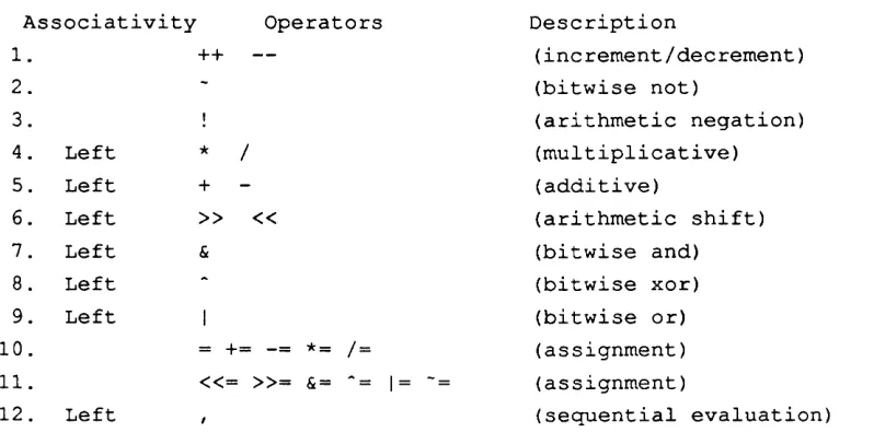
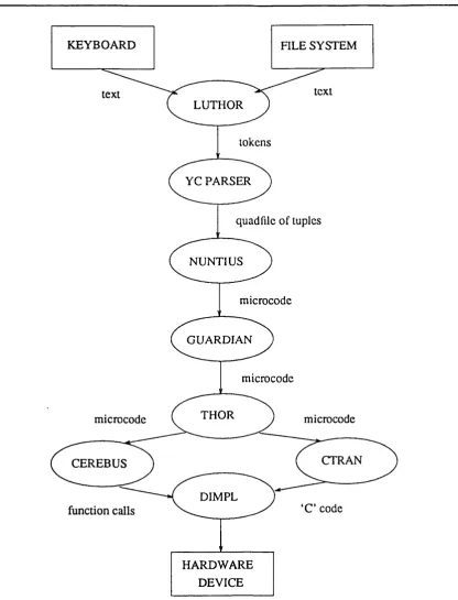
3.1 (table) YAM3D operators in order of decreasing p reced en ce________ 64 3.2 (table) A subset o f the grammar of Y A M 3 D _______________________ 65 3.3 Data flow through modules o f YAM3D __________________________ 67 3.4 Use o f lex and yacc in Y A M 3 D __________________________________ 70
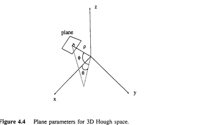
4.1 Spatial image together with log o f Fourier spectrum _______________ 83 4.2 Line parameters for 2D Hough space ____________________________ 84 4.3 2D Hough transform ______________________________________________ 85 4.4 Plane parameters for 3D Hough sp a c e ____________________________ 8 6
4.11 Butterworth fu n c tio n _________________________ _________________ 95 4.12 Serial section slices through a rats kidney ________________________ 97 4.13 Orthogonal slices and projections of slices in figure 4.12 ___________ 98 4.14 2D and 3D average filte r s _________________________________________ 99 4.15 2D and 3D median f i l t e r s ________________________________________ 101 4.16 2D and 3D expand f i l t e r s _________________________________ 103 4.17 2D and 3D shrink f i l t e r s _________________________________________ 104 4.18 2D and 3D closing _________________________ 105 4.19 2D and 3D o p e n in g ______________________________________________106 4.20 2D and 3D top-hat filter __________________________ 107 4.21 2D and 3D extremum f il te r s ______________________________ 108 4.22 2D Jannson-van Cittert deconvolution ___________________________ 111
5.1 First and second directional derivatives __________________________ 125 5.2 4-neighbour Laplacian and zero-crossings _________________________ 128 5.3 8-neighbour Laplacian and zero-crossings _________________________ 128
5.4 4-neighbour Laplacian and zero-crossings _________________________ 129 5.5 8-neighbour Laplacian and zero-crossings _________________________ 129
5.6 Ordered response o f 8-neighbour Laplacian _______________________ 130
5.7 Absolute value of Laplacian strength ranges for figures 5.8-9 _______ 131 5.8 M ulti-level 4-neighbour Laplacian _______________________ 132 5.9 Multi-level 8-neighbour L a p la c ia n _________________________ 132
5.10 Example neighbourhood for proof o f property III _________________ 138
6.1 (table) Half-space parameters and percent change _________________ 149 6.2 Plots o f sample slices through the half-spaces _____________________ 150 6.3 (table) Half-space signal-to-noise ratios and a of noise _____________ 151 6.4 (table) Ellipsoid parameters and percent c h a n g e ___________________ 151 6.5 Plots o f sample slices through the e llip so id s_______________________ 152
6 . 6 (table) Ellipsoid signal-to-noise ratios and a of n o is e ______________ 153
6.7 Resultant merit values for 2D and 3D g ra d ie n t________________ 154
6 . 8 Resultant merit values for 2D and 3D Roberts’ cross __________ 156
6.9 Resultant merit values for 2D and 3D Prew itt’s m a s k s _________ 157 6.10 Resultant m erit values for 2D and 3D Sobel’s masks ______________ 159 6.11 Resultant merit values for 2D and 3D Laplacian m a sk s_____________ 160
7.2 Idealised slice through carotid body _____________________________ 169 7.3 Stages in processing of bone data ________________________________ 170 7.4 YAM3D source code for bone extraction _________________________. 171 7.5 Stages in processing o f brain data _________________________________ 172 7.6 YAM3D source code for brain extraction ________________________ 174 7.7 Stages in processing of renal corpuscle data ______________________ 175 7.8 YAM3D source code for renal corpuscle e x tra c tio n _________________ 177 7.9 Stages in processing of carotid body data __________________________ 178 7.10 YAM3D source code for carotid body extraction __________________ 180 7.11 Scenario for failure o f the slice registration technique used __________ 181 7.12 (table) 2D 4-adjacent analysis re s u lts _______________________________182 7.13 (table) 3D 6-adjacent analysis re s u lts _____________________________ 182
7.14 (table) 3D 26-adjacent analysis re s u lts ____________________________ 183
8.1 Contour with chain code and run-length encoding ___________________ 186 8.2 Contour segments, spans, and graph representation __________________ 188 8.3 Acceptable and non-acceptable su rfa c e s ___________________________ 188 8.4 Toroidal graph representation ____________________________________ 189 8.5 Tetrahedral volumes ______________________________________ _ _ 191
8 . 6 Christiansen’s contour transform ation_____________________________ 192
8.7 Match g r a p h ___________________________________________ 194
8 . 8 Tiling te m p la te _______________________________________ 195
Acknowledgements
The author is indebted to the members of the Image Processing Group for provid ing a congenial working environment as well as many helpful suggestions. In particu lar I wish to thank my supervisor, Michael Duff, whose door was always open, and Mike Forshaw, Terry Fountain, David Greenwood, and Alan Wood, whose insights and experience contributed to this thesis.
I am also indebted to my parents, for providing both financial and moral support, and my wife, Helen, without whose patience and encouragement this work would not have been possible.
Chapter One: Introduction
A chronological progression from one-dimensional signal processing to two- dimensional image processing and later to three-dimensional voxel processing has taken place over the past thirty five years. Currently all three domains are active areas of investigation. The evolution of concepts from the one-dimensional signal realm to the image realm has been gradual and rigorous. Unfortunately such a successive refinement has not occurred from image to voxel processing, but rather a hiatus has taken place. This is partially, if not wholly, due to the rapid adoption o f voxel acquisi tion techniques in the field o f medical imaging, together with dramatic increases in availability and affordability of computers possessing significant processing power. The application o f image processing dates back to the ’50s and voxel processing to the early ’70s if not before. Surprisingly, in the twenty or so years since voxel processing first entered the scene, an analysis o f the differences between operating on voxel slices using image processing techniques versus using voxel processing techniques has not been published. O ther issues such as "is it possible to slice three-dimensional objects such that their resultant topology is incorrect" and "what is the ‘best’ surface detection operator" have not been addressed either.
This thesis attempts to address the lack of understanding between two-dimensional image processing and three-dimensional voxel processing in order to fill in the gaps in theory. In particular the focus of this thesis is to investigate the differences between operating on three-dimensional voxel data slice-by-slice, as if it were two-dimensional, and operating on it simultaneously using all three-dimensions within the domain of image/voxel processing. The intention is to cast the domain o f image and voxel pro cessing into a common theoretical framework, where voxel level operators are derived from commonly applied pixel level operators such that differences in extension as well as application can be determined.
such as a colour or texture.
M any of the ideas investigated and demonstrated appear to an expert to be "obvi ous" and "simple", and thus as a result have not been proven or demonstrated before, but rather, it appears, overlooked and taken for granted. It is hoped by the author that this work will lay a foundation for future, more in-depth investigations, as well as pro viding suggestions and ideas for approaching three-dimensional data. In the process it supports some work previously performed by others whilst dispelling myths in other approaches. Returning to the previous analogy, it is hoped that a coarse sketch of the jigsaw puzzle has been produced which will allow for successive refinement of the
pieces into the ultimate 1 0 0 0 piece puzzle.
The presentation and investigation o f ideas has a bias towards medical imaging applications, though the concepts covered pertain equally to most other voxel process ing domains such as the earth sciences. The focus on medical data is deliberate in that, it is hoped, the results and view o f this work will give guidance as to the "best" approach to the computer processing o f voxel data in a field on which human longevity may well come to depend.
Each chapter presents ideas already determined by others, as well as adding some thing new. On their own, these ideas are not major, but placed together in the frame work o f this unified view, contribute to the whole picture. Briefly, the contents of this thesis are as follows.
Chapter 2 is concerned with the physical and mathematical properties of voxels. In the process o f surveying acquisition techniques, physical and digital properties, and in investigating relationships between pixels and voxels, a solution to the well known three-dimensional connectivity paradox is presented. This solution is believed to be original, and is derived within a novel investigation into the morphological properties o f digital cells. Particular emphasis is placed on three-dimensional binary digital topology, where considerable research by others has already been performed. The detail presented is sufficient to allow for comparing differences o f operator output with respect to resultant topology in subsequent chapters.
Chapter 3 describes a simple yet powerful image and voxel processing environ ment which has been implemented to provide the necessary functionality for the majority of computer processing required in this thesis. As a result, it provides a com mon algorithm description language, at the slice level, which is used in subsequent chapters to describe the application o f operators to real and synthetic data.
providing numerous examples which demonstrate the differences between them with regards to resultant topology. Image operators such as transforms, filtering, and the like are described, extended to three-dimensions, and applied to real world data. This chapter covers significant ground and thus is a survey in the broadest sense.
Chapter 5 looks at the problem of edge and surface detection in detail, and in the process provides several new properties and theorems about the Laplacian operator which suggest under what conditions it can be successfully applied and what form is most appropriate for a desired resultant topology. The theorems and properties are believed to be original and are derived in an examination o f the output of the Laplacian within the context o f mathematical morphology. New, more accurate approximations to the three-dimensional Laplacian are also derived and presented. Inherent differ ences between the two- and three-dimensional operators are also described, thus pro viding a starting point for the application and analysis which follows in the next two chapters.
Chapter 6 looks at the performance of the operators derived in chapter 5 in the
presence o f noise under varying slicing conditions. It comprises an extension to an experim ent published over twelve years ago [Pratt78], which consisted of a com parison o f a class of two-dimensional edge detection operators. The new investigation presented herein consists o f comparisons between operators of different dimensionality as well as between the same dimensionality. In other words this chapter attempts to answ er the question as to which operator in a small class of surface detection operators is "best" under certain conditions. In the process o f answering this question the differ ences o f performance between two-dimensional operators and their three-dimensional counterparts is also examined.
Chapter 7 applies the "best" operator found in chapter 6 to various real world
voxel data sets and suggests an interesting perspective on how the output o f a surface detection operator can be used. The real data used contains various properties, ranging from desirable to undesirable. The purpose o f this work is to provide examples o f how such an operator can be applied, together with support from some o f the other filters described in chapter 4, and not actually to solve particular applications.
The display o f three-dimensional data is inherently more difficult than that of two-dim ensional images. As a result, chapter 8 surveys different solutions to the prob
lem o f displaying three-dimensional voxel data. Demonstrations o f some o f the m ethods are given on the segmented real world objects described in chapter 7. Chapter
8 also presents a new pattern recognition approach to the fitting of polygons to sur
The order and contents of the chapters has been chosen to facilitate a gradual spiral from abstract to specific, from general to particular. As a result, the ordering of operators presented is not necessarily chronological in terms o f how they might be typ ically applied. This particular ordering has been chosen to build up momentum in get ting to the analysis of a particular class of operators in chapters 6 and 7. Therefore,
Chapter Two: Voxel Data
This chapter is concerned with both physical and mathematical properties of two- dimensional (2D) and three-dimensional (3D) image data sets. An understanding of these properties is essential if meaningful operations are to be performed. In a sense this chapter is the foundation upon which subsequent chapters rest.
The chapter is divided into four sections. The first sets the stage by describing the digital form o f both 2D and 3D data sets. The second section surveys how these data sets are acquired, what information they contain, and the forms of error which crop up in their acquisition. The third section defines important mathematical properties of discrete digital data which must be taken into account when performing processing and analysis. Also a new detailed investigation into digital adjacency as it applies to cell morphology is presented which culminates in a new, definitive solution to the 3D con nectivity paradox. The final section examines the relationships between 2D and 3D images and, in the process, makes an analogy to computer graphics rendering and minimum sampling conditions.
2.1 Theoretical foundations
2.1.1 Two-dim ensional intensity function
represents. It is often useful, as we shall see in locating edges and surfaces, to consider the image to be an approximation to a 2D function / 2(x , y ) where the X and Y dimen sions are generally treated as orthogonal basis vectors in the Euclidean space R 2, and the value of the function at a particular point is considered to be a measured intensity.
Depending on the field o f application, image processing can be an extremely difficult task, since images are often just a projection o f a 3D scene. The depth infor mation implicitly contained within an image includes occlusions, focus, perspective, texture, a priori knowledge o f object sizes, and perhaps shadows.
2.1.2 Three-dimensional density function
Techniques to acquire truly 3D images have been developed to circumvent the difficulties associated with making depth measurements using conventional 2D image processing techniques. Aside from issues such as depth, occlusions, and shadows, information concerning the interior structure of many types of 3D scenes has been found to be useful. Consider for example the need to accurately identify the location o f a blood clot or tumour within a human body non-destructively, i.e. without perform ing unwanted and perhaps dangerous in-vivo exploratory surgery.
Sometimes binocular stereo image pairs are used and computer analysis is per formed to reconstruct depth information. This approach is similar to that used by bio logical visual systems such as those o f man and reptile. Although great strides have been made in stereo imaging, information on the interior o f objects is not available and both occlusions and shadows can still occur, and thus it can be thought o f as an intermediary step between 2D processing and 3D processing.
A function analogous to, but somehow differing from, / 2U ,y ) exists for 3D data
sets, nominally referred to as voxel data sets. The function / 3(jc ,y ,z ) o f three dimen
sions is usually defined over orthogonal spatial axes o f the Euclidean space R3 and
consists of some measured attribute o f the original 3D scene such as the density of a material present within a volume surrounding each point (.x ,y ,z ).
2.1.3 Digital representations
W e shall refer to the digital representation of / „ in R n as Z n . In Z n we refer to the elements making up the grid as unit cells or just cells. In 2D a cell is a pixel and in 3D a cell is a voxel.
A t first glance the differences between the functions Z2 and Z3 are straightforward
and result from the addition o f a new dimension. For example, Z3 spans a 3D space
rectangle. Z2 is subdivided into 2D rectangles (pixels) and Z3 is subdivided into 3D
hexahedra (voxels). Lastly, a pixel typically represents that percentage o f reflected and refracted energy from the scene being imaged which converges in a small rectangle, while a voxel usually represents the percentage o f energy contained within a hex ahedron within the scene being imaged. As is the case with two dimensions, the voxel data set acquired consists only of a discrete approximation to the original continuous scene, and thus consists o f numbers quantised at a limited number o f integer values within a range o f a possible set o f values consisting o f a power o f two, with exponents
1, 8, and 16 and being the most common.
The remainder of this chapter will focus on physical methods used to generate Z2
and Z 3 from / 2 and / 3 and will investigate digital relationships in Z2 and Z3 and in so
doing uncover further differences between them.
2.2 Physical p ro p erties
2.2.1 S ources of voxel d ata
V oxel data sets are generated in applications from a wide spectrum o f fields, among them being the rapidly advancing field of medical imaging, the biological sci ences, seismology, fluid dynamics, meteorology, structural engineering and geology. M ost voxel acquisition procedures fall into two broad methods. One o f these methods involves transmitting some form o f energy through a 3D medium and measuring and recording the energy which is emitted. The second category involves measuring and recording energy which is either inherent in a medium or has been artificially induced. W e shall refer to these categories as active acquisition and passive acquisition respectively.
samples also using CT reconstruction methods. Examples of passive techniques are single photon emission computer tomography (SPECT), multicrystal positron emission tomography (PET) and emission computed tomography (ECT). These techniques involve the injection o f a radio-isotope and subsequent measurement of the emitted energy, usually gamma rays, in ID slices which are then also reconstructed using back projection methods to yield 2D slices.
There exists an active acquisition imaging technique, used in the biological sci ences, which is not performed in-vivo and does not use back projection. The 2D slices are called serial sections. In this case, the objects o f interest are physically sliced into thin parallel 2D planes and are stained and imaged, sometimes under a microscope, where the energy transmitted and recorded is that o f visible or ultra-violet light.
In the previous examples we have seen that various forms o f energy are used and measured. The wave motion o f particles in a medium such as water or air can also be measured, such as is in fluid dynamics and meteorology. In geology and seismology, shock or sound waves are induced and measured as they pass through, and are reflected off, materials.
The data used to illustrate the techniques derived in subsequent chapters consists o f samples derived from active acquisition processes, namely MRI and serial section microscopy. Phantom data is also generated and used. A description of the acquisition and generation o f the voxel data used can be found in Chapters 6 and 7.
Detailed information on the physics o f voxel acquisition is beyond the scope of this thesis. Interested readers are directed to [W ebb8 8] for a discussion of the physics
o f medical imaging. In particular for x-ray computed tomography [Dance8 8],
[Evans8 8], [Swindell8 8], and [Dobbs8 8], for radio-isotope imaging such as PET,
SPECT, and ECT [Ott8 8], and MRI [Leach8 8] which also gives a detailed introduction
to the process o f CT back projection techniques. Detailed theory and application of CT back projection techniques can be found in [Herman80], [Barret81] and [Natterer8 6]. For the physics o f the interaction o f light such as is used in laser ranging
and serial section microscopy the reader is directed to [Jenkins81] and for wave propa gation such as is used in diagnostic ultrasound, seismology, and fluid dynamics to [Bamber8 8].
2.2.2 Inform ation content in voxels
More specifically, a voxel is a volume element containing a discrete density value which represents some measurable physical phenomenon, usually corresponding to the interaction between energy and material in a constrained volume of space. In the case o f MRI data it is the proton densities and spin echo; in serial sections it is the interac tion o f light characterised by reflection, transmission, and refraction. The range of pos sible voxel values represents the relative degrees o f energy interaction over some spec trum o f measurable phenomena. It is usually correlated with physical densities so that a small value represents no object, and a large value the surface or interior o f an object. For example, in the case o f serial sections, large density values are portions of anatom ical structures such as arteries and low values are the surrounding medium, whether tis sue or fluid.
Since the human visual system is only appropriate for the visualisation of 2D pro jections of 3D scenes, voxels are generally derived as a visualisation aid to understand ing, such as diagnosing and measuring the internal nature o f various 3D objects. In the case o f the medical sciences, the benefits are obvious as internal structures can be non-destructively measured in-vivo. In the physical sciences massive structures, such as portions of the earth’s crust, can be studied without large scale excavation and des truction.
Voxels are ordinarily considered to be cubic, although one o f its three dimensions may sometimes be larger than the other two. The corresponding real world dimensions o f a voxel are dependent on the specific acquisition method used, and range from mil limetres and centimetres for medical imaging and serial section microscopy, to metres and kilometres or more for geology, seismology, and meteorology.
With some idea o f what information a voxel represents, its dimensions, and the significance o f its digital value, which we will hereafter refer to as its grey-level, we can now examine the sources and effects of noise in voxel data sets.
2.2.3 Noise
Penum bra is a form of noise in the resultant image due to the finite size of some energy source, such as x-rays (of wavelength 10- 1 nm). The blurring B in an image
can be calculated geometrically for a point energy source as follows, where m is the image magnification, W the aperture width o f the collimator, d i the distance from the collim ator to the energy source, and d2 the distance from the collimator to the image
plane (see figure 2.1).
The important thing to note about penumbra is that the amount of blur is related to image magnification and to the size of the collimator being used.
Figure 2.1 Geometrical calculation o f blur resulting from penumbra.
Statistical fluctuations in the energy detected by receptors can result in fluctuations in the digital signal being recorded. These fluctuations result in small changes in the apparent density o f a voxel, and thus a homogeneous region ends up being represented as a heterogeneous digital region. Such fluctuations can in principle be clamped to be within a narrow range by increasing the energy dosage. Since increase in energy dosage is not always feasible, as its effect may be harmful to the subject or the
B = W 1 + 4 2- =W (l+m )
Blur B detector
(image plane)
W\ collimator
receptors, various forms o f computer processing can be performed to blur and average such effects. Processing of this form is described in more detail in Chapter 4.
Scatter is characterised by fluctuations in the amount of energy absorbed by the receptors as it is emitted from the scene being imaged. In active acquisition methods, scatter results from the fact that the energy applied does not in general intersect the objects in its path at precisely right angles. A small deviation in the angle results in a receptor close to the correct one detecting the energy and a large deviation results in a receptor quite far away detecting the energy. The overall effect o f scatter is to intro duce ‘salt and pepper’ noise to the discrete data and to blur what might otherwise have been sharp edges.
The last internal acquisition error factor is receptor resolution. Since energy will diverge in directions out o f the current slice plane an energy beam measured in one direction may be recorded at a slightly different position and value to a beam in the opposite direction.
Background noise consists o f energy collected from the environment at large. A real world example is the white noise sound emanating from some electrical appli ances, which interferes with an otherwise clear radio signal. Background noise o f this type is also exhibited in the form of salt and pepper noise.
Blurring and misregistration, due to object movement whilst the imaging process is taking place, or due to miscalibrated receptor planes, is a common phenomenon. A lthough reducing the time o f physical data acquisition when possible will reduce its effect for medical imaging, the problem is inherent in serial section microscopy. Serial sections are typically laid out on a microscope slide as they come out of the micro tome. As a result computer processing must be applied to register (align) each slice with its previous and next neighbours. Although it is theoretically possible to do this to an accuracy within ±Vi a voxel, in practice this is not always the case. Issues related to slice registration are discussed in Chapter 7.
Tom ographic reconstruction itself can be a source of error as well as a magnifier o f errors that have crept into the imaging process prior to its application. As an exam ple phantom edges and shadows are known to be produced [Leach8 8]. One reason for
this is that information is being interpolated from sometimes sparse samples.
in inter-slice noise.
2.2.4 Contrast and sharpness
O ther manifestations of noise in voxel data sets include low levels of contrast and some degree of unsharpness in digitised objects. Contrast is affected by the resolvable accuracy o f the measurement device, discretisation o f the density property being meas ured, and the local properties of the scene. Consider for example how varying amounts of bone, fat, and fluid can affect resultant measurements. The effective resolution of the detector being used for measurement, as well as the scattering effect of the objects being im aged for a particular form of energy (photons for example), can play substan tial roles in reducing the sharpness of the resultant data.
Considerable improvements are being made by medical imaging technologists in reducing the background scatter recorded by detectors. Physical improvements include the use o f devices such as scanning slits and both stationary and moving grids. Another improvement involves minimising the separation between the patient and the receptor device, thus taking advantage of the well known inverse square law. The inverse square law simply states that the magnitude of the signal falls off as the inverse of the square o f the distance between the object being imaged and the receptor. The general idea behind all these techniques is to record only that energy which is as close to perpendicular as possible to the imaging medium. Computerised techniques are also applied to increase sharpness. One medical practitioner states "without image decon volution, the tomographic data are too confused to be o f much use."f
2.2.5 Spatial dependencies
Inaccuracies in the digitisation of a defined region in the original scene will, in general, result in inaccuracies in the corresponding voxel in the digitised image and also in that voxel’s immediate neighbours. Consider for example, the digitisation o f a solid surface, where the quantity measured and recorded for each voxel corresponds very closely to the percentage or amount o f the original solid surface contained within the corresponding real world volume of the voxel. For a given voxel, the boundary or edge o f the surface might exactly cover only half o f the voxel, and thus results in a digitised voxel’s value of one half. If we then include some o f the possible forms of error previously discussed, we may find that the density value will also vary slightly from the true fifty percent say, because of scattering effects from neighbouring voxels
entirely contained within the interior of the object. When cases such as this are looked at on a slice-by-slice basis, one sees that the edge o f the surface for that slice is fuzzy.
A nother type o f unsharpness occurs when the objects that are being imaged move faster than the image scan time of the imaging device. This results in the measured density being blurred over the time of the movement and is called motion blur. For example, in photography the use of a slow shutter speed on fast moving objects results in the moving objects being smeared across the image. Depending on the speed of motion and the apparent size o f the moving objects with respect to the resultant photo graph, the smear size for a given point ranges from local neighbourhood regions to long streaks possibly covering the entire photograph. In medical imaging patient respiration, the beating o f the heart and blood flow can cause such effects.
In each o f the aforementioned cases we see that the blurring effect is predom inantly localised over a local neighbourhood for a given voxel. Other situations also exist, such as where extremely dense portions o f the original scene emit more energy than less dense portions. This energy is scattered and recorded in neighbouring, less dense voxels. Situations such as the above must be corrected, or at least accounted for, when analysing and finally presenting measured properties o f the voxel data. In the case o f serial sections, the initial stage of digitising the slices must align (register) the slices so that they may be treated later as a 3D data set.
2.3 Digital properties
H aving a mathematical formulation of a 3D scene / i(x ,y ,z ), an understanding as to how its discrete digital approximation Z3 is represented, where voxels come from,
and the types o f error that are likely to appear in the process o f acquisition, we may now investigate several important concepts which must be considered when operating upon Z 3.
2.3.1 Square/cubic adjacency
In one dimension, a configuration o f cells is said to be sym m etric if it is equivalent to itself rotated by an angle of n. In ID we need only consider a 3x1 neigh bourhood if we are interested in knowing when cells are adjacent, because a cell has only two neighbours in ID. In a 3x1 neighbourhood there are four unique symmetric configurations of cells, as in figure 2.2.
F ig u re 2.2 Symmetric ID adjacency configurations.
A graphical representation of adjacency sets is used, where a black cell indicates that the cell contains an object value and a blank cell indicates a background value. Throughout the rest of this discussion adjacency sets are defined for black object cells as a notational convenience. O f the ID configurations, a definition o f adjacency need only consider those whose central cell together with one of its neighbours contain an object value. We define such a configuration to be reasonable. Thus we can see that there is only one ID reasonable symmetric adjacency set which is D 1 and which con
sists o f a cell together with its two neighbours. M oreover we can see that half of the configurations are the inverse of the other half, namely those where A 1=—iD1 and B 1= —iCl . If we call the directions of D1 left and right, then given a cell a and another
cell p, p is 2-ad jacen t to a if p touches a on either its left or right side.
B2 C2 D2 E2 F2
F ig u re 2.3 Symmetric 2D adjacency configurations.
From figure 2.3 we see that there are three symmetric neighbourhood configurations for 2D which are reasonable. These adjacency sets are F 2, G 2, and H2
where we shall refer to the relationships that they represent as 4-adjacency, 4 ’- ad jacen cy , and 8-adjacency respectively. 4 ’-adjacency is rarely used, as it considers
pixels to be adjacent which intersect in less area than other possible neighbours (i.e. they touch only in a vertex as opposed to an edge). The 4-adjacency set is sometimes referred to as the von Neumann neighbourhood and the 8-adjacency set as the Moore
neighbourhood.
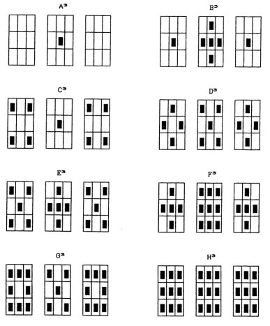
3D symmetry implies rotational invariance about an angle of -j*, only now about three axes rather than two. The 3x3x3 neighbourhoods of voxels can be derived using the same technique as that used in deriving the 2D configurations from the ID configurations. Instead o f using the ID edges though, we let each 3x3 face be one of the 2D configurations. Again a copy of the eight 3x3x3 configurations is made with the central voxel either empty or full. Eight of the sixteen 3D symmetric 3x3x3 voxel neighbourhood configurations are shown in figure 2.4 in the form of consecutive 3x3 slices through the cubic neighbourhood. The remaining eight configurations are the same but with the central voxel blank.
O f the configurations in figure 2.4, B 3, F3, and H3 are the most commonly used
and are referred to as 6-adjacency, 18-adjacency, and 26-adjacency respectively. The
other configurations are not generally used, as they define neighbouring voxels to be adjacent, which share less common surface area with the central voxel under con sideration than other neighbouring voxels which they define as being non-adjacent.
E3
G3
1
1
1 1
1
1
1 1 1
1
1 1 1
1 1 1
1 1 1
D3
F3
Figure 2.4 Symmetric reasonable 3D adjacency configurations.
reasonable symmetric adjacency sets then are 4-adjacency and 8-adjacency and in 3D
they are 6-adjacency, 18-adjacency, and 26-adjacency.
4-adjacent and 8-adjacent. In 3D, two voxels which share only a common vertex are
26-adjacent, two that share only a common edge are both 18-adjacent and 26-adjacent, and two voxels that share a common face are 6-adjacent, 18-adjacent, and 26-adjacent.
2.3.2 Connected components and curves in Z n
It is difficult to ascertain the originator(s) o f the definitions and terminology which follows in this section and the next. The choice of terms and definitions used here is modelled closely after [Rosenfeld77].
A notion o f connectivity is fundamental to any definition o f an object in Z " . A continuous real world object, when digitised, should result in a discrete connected object if any meaningful measurements and analysis are to be performed. A digitised object must then consist of a set of adjacent points. However, it has been shown that there are several possible definitions of how digital cells can be considered to be adja cent. For the moment, let us discuss the general case, and assume that one of the previ ous adjacency sets has been chosen and define what it means for an object to be con tinuous in the discrete sense or, more precisely, connected. In the following, we assume that the contents of the cells take only the values ‘black’ and ‘white’.
Two cells a and (3 which are elements o f a set V are said to be connected if there exists a sequence o f members a=PotP i , . . . , Pm- (3 such that each Pi is n-adjacent to
P i -1 for 1 <i<m and P / e T for 0<i<m. The sequence o f members Pq, . . . ,P m is
called a path. A homogeneous set of cells is said to be a connected component or just a component if every element of the set is connected to every other element of the
set. A component defined using n-adjacency is said to be n-connected.
In order to differentiate one component from other components, the process which is called segm entation, we must define whether a cell is in the interior of a component or on its border. A cell is said to be isolated if the com ponent of which it is a member consists o f no other cells. Thus an isolated cell is not adjacent to any other cells o f the same value. A cell is called a border cell if it is adjacent to a cell o f a different value. Thus an isolated cell is a border cell but a border cell is not necessarily an isolated cell. If a cell is not a border cell then it is an interior cell, and thus all o f the adjacent neigh bours o f an interior cell have the same value as the interior cell.
2.3.3 Frontiers and holes
A component £2 surrounds another component *F if and only if every border cell of *F is adjacent to a border cell of £2. The notion of surrounds should not be confused with ‘encompasses’ as the former requires that the components touch. A component can be both surrounded by a component and surround a component. For example £2 may surround 'F and *F may surround T. For this to occur, £2 does not surround T, but rather it encompasses it. If £2 and T consist of background values then T is called a hole if it is 2D and is called a cavity if T is 3D.
The area of intersection of £2 and 'F (i.e. the shared voxel faces of border cells in both £2 and 'F in Z 3) when £2 surrounds *F is said to be the frontier between £2 and XF. More specifically this frontier is called the outer frontier o f 'F and an inner frontier of £2. If £2 surrounds other components then it has several inner frontiers. The outer frontier o f a 2D component is its perimeter and o f a 3D component is its outer surface.
If a closed curve has exactly two frontiers it is said to be a sim ple closed curve, if it has only one frontier (eg. a 2x2 square o f pixels) is said to be a degenerate closed
curve, and if it has more than two frontiers (eg. a figure eight) then it is called a com plex closed curve.
2.3.4 Connectivity paradox
In 2D a component is sometimes referred to as a region and in 3D as an object. A region consists o f a set o f connected pixels, both border and interior, which is assumed to entirely consist o f the real world ‘object’ in / 2 which has been digitised. Similarly
an object consists o f a set of connected voxels which is assumed to consist entirely of the real world ‘object’ in / 3. Definitions for the surface (perimeter) o f an object
(region) have been given without considering adjacency relationships. The adjacency used was assumed to have been chosen for our definition of connectivity.
A paradox exists when choosing one o f the many adjacency sets previously derived. This paradox was initially pointed out for the 2D case by Rosenfeld and Pfaltz in [Rosenfeld6 6]. In figure 2.5, if all pixels (both background and region) are
taken as being 4-connected then the black pixels are disconnected (and thus consist of four components), yet they still divide the white pixels into two separate components. If all pixels are assumed to be 8-connected then the black pixels form a single com
Jordan curve theorem states that a simple closed N-dimensional curve in an N- dimensional space will divide the space into two separate components.
Figure 2.5 Connectivity paradox in 2D.
The resolution to this paradox was proposed by Duda et al in [Duda67] and is rather straightforward. If we consider objects to be black and background to be white then we must use opposite connectivities for each. For example, if we take the black objects in the previous figure to be 8-connected and the background to be 4-connected,
then the Jordan theorem holds, that is the black curve divides the space into two non connected regions of background. Similarly, if we choose the black pixels to be 4- connected and the white pixels to be 8-connected, then there are four black com
ponents and only one white component.
The connectivity paradox is much more subtle in 3D. The resolution of the 3D paradox is to use 6-connected object cells and either 18-connected or 26-connected
background cells [Rosenfeld81]. Similarly if either 18-connected or 26-connected object voxels are used then the background must be treated as being 6-connected. For
example, if in figure 2 . 6 the black voxels are taken as being 18-connected, then the
background must be 6-connected, otherwise the cavity seen as a hole in the central
slice will be connected to the background with either an 18-connected or a 26- connected background.
2.3.5 Hexagonal/dodecahedral adjacency
Hexagonal pixels, rather than rectangular, are sometimes used to circumvent the 2D connectivity paradox, yielding 6-connected regions on a 6-connected background
1
i 1 1 1
1
F ig u re 2.6 Connectivity paradox in 3D.
rectangular pixels become the defacto hardware standard for display. One scheme for simulating hexagonal 6-connectivity in software involves using standard rectangular
pixels, but treating alternate rows as if they had been shifted by half a pixel. For exam ple, if odd numbered rows are to be ‘shifted’ to the left then the connectivity configurations are in figure 2.7, where E2 is used on even numbered rows and O 2 on
odd numbered rows.
E* Oa
1 1 1 1
1 1 1 1 1 1
1 1 1 1
F ig u re 2.7 Shear masks for hexagonal connectivity.
Like the cube, the dodecahedron is a regular congruent polyhedron, and like the hexagon, the edge angle between faces meeting at a vertex is 120°. A polyhedron is a solid which is bounded solely by planar faces. A congruent polyhedron consists of polygonal faces which are all o f the same size and shape. A polyhedron (polygon) is convex if connecting line segments between every pair o f vertices lies solely inside, or on the edge of, the polyhedron (polygon).f A convex polyhedron is called regular or Platonic if it is bounded by congruent polygons in which the same number of edges meet at each vertex.
The dodecahedron can be simulated in a cubic grid by shearing. First alternate columns are ‘shifted’ by half a pixel, then alternate slices by the same. For example, if odd numbered columns are to be ‘shifted’ to the left, and even slices down, then the connectivity configurations are as in figure 2.8, where E 3 is used on even numbered slices and O3 on odd numbered slices.
E3
Figure 2.8 Dodecahedral shear masks.
The connectivity paradox is averted in both cases, since no two adjacent cells share a common border which is of less area in any other direction. Put another way, in each case every vertex on the frontier of a cell is shared by exactly three adjacent cells, where the angles between the faces from which it is made are precisely 1 2 0°; all adja
cent cells touch in an edge in 2D and a face in 3D.
2.3.6 Connectivity and discretisation error
Apart from the connectivity paradoxes described above, there are other issues which play a role in selecting a connectivity. These issues include algorithmic com plexity in traversing a 3D surface, and how actual objects are represented when digi tised. If we accept the algorithm o f a walk of a 26-connected surface as possible, though somewhat difficult to implement, then the representation o f true continuous objects in voxel space must be considered.
Consider for example the simple 2D case of a thin cross. If the axes of the cross lie nearly on the digitisation axes of the grid, then the resulting region will be accu rately represented using a 4-connected definition. Unfortunately, if the cross is rotated by forty-five degrees from the axis of the digitisation grid, the resultant representation at the crossing of the lines will be distorted. The distortion error will be small for a well sampled cross (i.e. where a high resolution sampling grid has been used, so that the cross consists of many pixels) and large for a poorly sampled cross (consider a one pixel thick cross). For reasons such as this it is desirable to digitise at a resolution which is meaningful for the objects of interest to be analysed, i.e. above the Nyquist frequency.
Other interesting related artifacts which must be considered include the final representation of surfaces and edges. One example suffices to give a feel for these problems. Consider a digital line, which may be the final result o f skeletonising an object to its medial axis. Its 6-connected representation will on average consist of
many more voxels than its 18-connected or 26-connected representation, and thus be thicker. This also holds true for voxels making up surfaces, thus taking volume or per imeter measurements, by actually counting the number o f voxels, may result in dif ferent values for each possible connectivity.
2.3.7 Frontier tracking
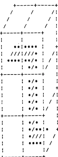
F ig u re 2.9 Voxel face nodes with both in-degree and out-degree o f 2.
A rtzy derived a border voxel tracking algorithm in [Artzy78] which was later, in [Herman83], proved correct and to terminate. Artzy proposed that the voxel represen tation o f Z3 be converted to a directed graph representation where for each face of a
voxel, two of its edges are labelled as in and the other two as out, such that each edge is an out-edge o f one face and an in-edge of another. Converting each voxel face to be a node and all of its edges to be arcs yields a directed graph, where for each 6-adjacent
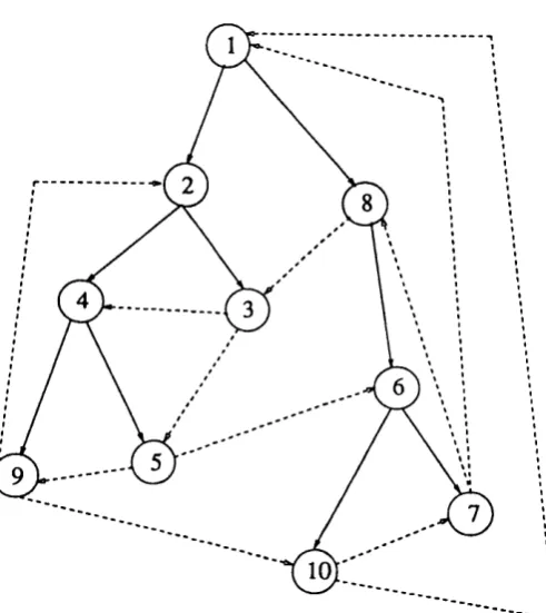
voxel we have six nodes, each containing four arcs and having an in-degree o f two and an o u t-d eg ree of two as shown in figure 2.9. The in-degree (out-degree) of a node is the num ber o f arcs entering (leaving) the node. Given this representation one can apply standard binary tree traversal algorithms to the graph to track its surface. Figure 2.11 shows both the binary tree and directed graph for the 3D object in figure 2.10. A rtzy proposed refinements to the tracking procedure to make it more efficient, since both the in-degree and out-degree are restricted to two. This adaptation is accom plished by processing the graph as a set o f lists rather than a binary tree. Further efficiency refinements have been developed and can be found in [Lobregt80], [Udapa82], and [Gordan87].
Z H
F ig u re 2.10 A 3D object with arbitrarily labelled surface voxel faces.
The difficulty with this method is that a different algorithm must be used to track the interior border as it consists of background voxels and thus, because of the connec tivity paradox, uses a different adjacency set.
2.3.8 C ell m orphology
So far we have defined several adjacency sets for both 2D and 3D. Before we can go on to consider both Euclidean and topological metrics of the cells represented by these adjacencies, we must have a better understanding of their ‘shape’. A shape can be assigned to a polygonal cell based on the number o f neighbours to which it is adja cent. These shapes are hypothetical, in that the cells are generally digitised and represented within a square or cubic grid and thus their digital shape is that of a square or cube. The hypothetical shape is a construct derived assuming that the shape o f the real w orld portion o f space that has been digitised is defined by the adjacency set used in operating upon it. This notion of shape is useful in that it allows for criteria to be defined which can help in deciding which adjacency set to use.
A 4-connected pixel is a 4 sided regular polygon, which is called a square when its edges are parallel to the X and Y axis. A 6-connected pixel is a 6 sided regular
polygon, which is called a hexagon when two o f its edges are parallel to the X axis, 7T
two o f its edges are rotated by an angle o f -j- with respect to the X axis, and two are rotated by the same angle with respect to the Y axis. An 8-connected pixel is an 8
Figure 2.11 Binary tree (solid lines) and directed graph (solid and dotted lines) for figure 2.1 0.
7T
the X axis, two to the Y axis, two of its edges are rotated by an angle of with respect to the X axis and two by the same angle with respect to the Y axis.
In 3D, a 6-connected voxel has the shape o f a cube (hexahedron), an 18-connected
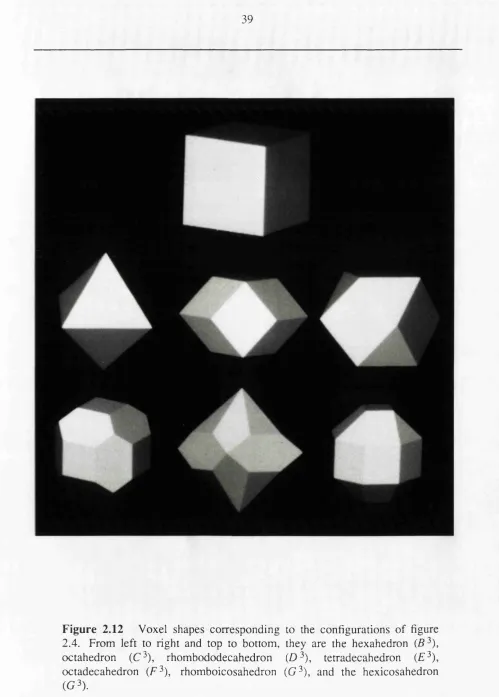
voxel the shape o f a octadecahedron, and a 26-connected voxel the shape o f a hexi- cosahedron. In Section 2.3.1 (figure 2.4) the other adjacency sets together with their shapes are: C 3, the 8 faced octahedron; D 3, the 1 2 faced rhombododecahedron; £ 3,
the 14 faced tetradecahedron (cuboctahedron); and G 3, the 20 faced rhom- boicosahedron. Properties of the tetradecahedron have been investigated in [Pres- ton80] and [Serra8 8] and the rhombododecahedron in [Serra8 8]. O f the symmetric
adjacency sets thus derived, the Platonic regular congruent solids o f the cube and octahedron can be used to tessellate a 3D space (though both still yield a connectivity paradox). The remaining tetradecahedron and hexicosahedron are Archimedian semi regular solids and can not be used to tessellate. A rchim edian (sem i-regular) solids do not have congruent faces, but all of their faces are regular polygons (i.e. they are composed of more than one type of polygonal face).t Although there exists a Platonic icosahedron, the twenty faced voxel generated from G3 is not regular and thus cannot
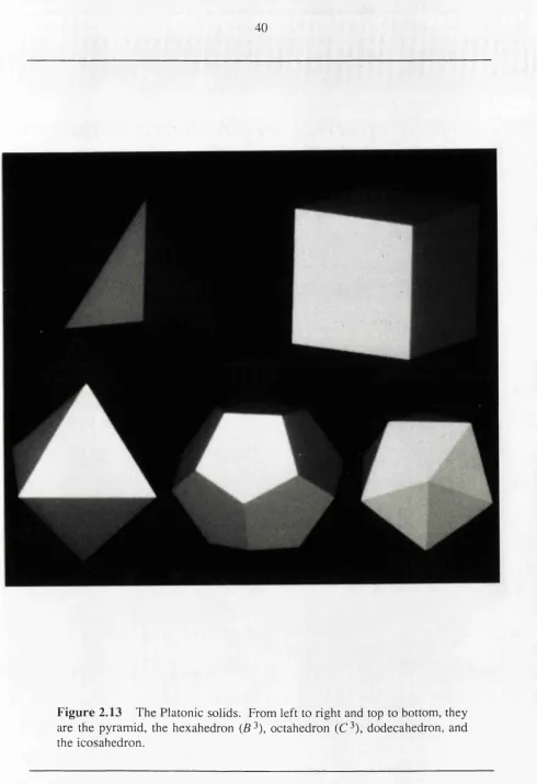
be used to tessellate three space. The shapes of all these voxels are as in figure 2.12. The Platonic solids o f figure 2.13 all tessellate 3-space. Among them the cube (hexahedron), octahedron, and dodecahedron have already been described. Since the 4 sided pyramid does not have a symmetric adjacency set it is not covered in this thesis. The twenty faced icosahedron is not considered either, because a connectivity paradox will occur with its usage since neighbouring voxels can be adjacent only in a vertex. Since this is the case the rhomboicosahedron may as well be used, as no shearing is required for its representation in a digital grid.
Plato’s proof that no other regular congruent polygonal solids exist (and thus no other 3D tessera) in 3D is straightforward; a sketch of the proof is as follows. If a polyhedron is bounded by equilateral triangles, then the edge angles are 60° and only three to five faces can meet at a vertex (since by theorem the sum of the edge angles at a vertex must be less than 360°). If a polyhedron is bounded by squares or regular pen tagons then only three can meet at a vertex (by a similar argument, since the edge angle is 90° for a square and 108° for a regular pentagon). Faces o f six sides (regular hexagons) and more cannot be used since each angle is greater than or equal to 1 2 0°.
Choosing a voxel shape other than the cube requires some thought as to what mor phological properties a voxel should have. Serra suggests four criteria for the selection o f a cell shape in 3D [Serra82]. These criteria are as follows.