This is a repository copy of
LASSO-Driven Inference in Time and Space
.
White Rose Research Online URL for this paper:
http://eprints.whiterose.ac.uk/165628/
Version: Accepted Version
Article:
Wang, Weining (Accepted: 2020) LASSO-Driven Inference in Time and Space. Annals of
Statistics. ISSN 0090-5364 (In Press)
[email protected] https://eprints.whiterose.ac.uk/ Reuse
Items deposited in White Rose Research Online are protected by copyright, with all rights reserved unless indicated otherwise. They may be downloaded and/or printed for private study, or other acts as permitted by national copyright laws. The publisher or other rights holders may allow further reproduction and re-use of the full text version. This is indicated by the licence information on the White Rose Research Online record for the item.
Takedown
If you consider content in White Rose Research Online to be in breach of UK law, please notify us by
LASSO-Driven Inference in Time and Space
∗Victor Chernozhukov†, Wolfgang K. Härdle‡, Chen Huang§, Weining Wang¶ May 18, 2020
Abstract
We consider the estimation and inference in a system of high-dimensional regression equations allowing for temporal and cross-sectional dependency in covariates and error processes, covering rather general forms of weak temporal dependence. A sequence of regressions with many regressors using LASSO (Least Absolute Shrinkage and Selection Operator) is applied for variable selection purpose, and an overall penalty level is carefully chosen by a block multiplier bootstrap procedure to account for multiplicity of the equations and dependencies in the data. Correspondingly, oracle properties with a jointly selected tuning parameter are derived. We further provide high-quality de-biased simultaneous inference on the many target parameters of the system. We provide bootstrap consistency results of the test procedure, which are based on a general Bahadur representation for theZ-estimators with dependent data. Simulations demonstrate good performance of the proposed
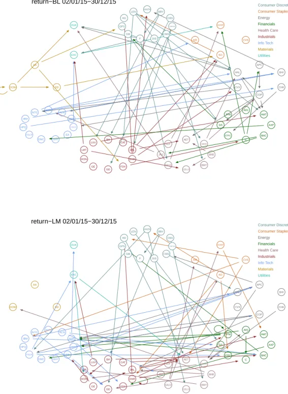
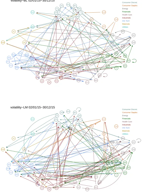
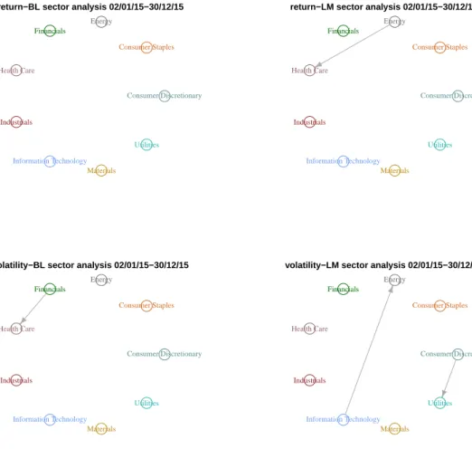
inference procedure. Finally, we apply the method to quantify spillover effects of textual sentiment indices in a financial market and to test the connectedness among sectors.
JEL classification: C12, C22, C51, C53
Keywords: LASSO, time series, simultaneous inference, system of equations,Z-estimation, Bahadur
representation, martingale decomposition
1
Introduction
Many applications in statistics, economics, finance, biology and psychology are concerned with a system of ultra high-dimensional objects that communicate within complex dependency chan-nels. Given a complex system involving many factors, one builds a network model by taking a large set of regressions, i.e. regressing every factor in the system on a large subset of other
∗We thank Weibiao Wu, Oliver Linton, Bryan Graham, Manfred Deistler, Hashem Pesaran, Michael Wolf,
Valentina Corradi, Zudi Lu, Liangjun Su, Peter Phillips, Frank Windmeijer, Wenyang Zhang and Likai Chen for helpful comments and suggestions. We remain responsible for any errors or omissions. Financial support from the Deutsche Forschungsgemeinschaft via IRTG 1792 “High Dimensional Non Stationary Time Series”, Humboldt-Universität zu Berlin, is gratefully acknowledged.
†Department of Economics and Center for Statistics and Data Science, Massachusetts Institute of Technology. ‡IRTG1792, Humboldt-Universität zu Berlin. School of Business, Singapore Management University. Faculty
of Mathematics and Physics, Charles University. Department of Information Management and Finance, National Chiao Tung University.
§Department of Economics and Business Economics and CREATES, Aarhus University. Corresponding
au-thor: [email protected]
¶Department of Economics and Related Studies, University of York. Ladislaus von Bortkiewicz Chair of
Statistics, Humboldt-Universität zu Berlin.
factors. Examples include analysis of financial systemic risk by quantile predictive graphical models with LASSO (Hautsch et al., 2015; Härdle et al., 2016; Belloni et al., 2016), limit order book network modeling via the penalized vector autoregressive approach (Härdle et al., 2018), analysis of psychology data with temporal and cross- sectional dependencies (Epskamp et al., 2018). Another example is quantifying the spillover effects or externalities for a social network, especially when the social interactions (or the interconnectedness) is not obvious (Manresa, 2013). Besides, there are numerous applications concerning association network analysis in other fields of applied statistics; see Chapter 7 in Kolaczyk and Csárdi (2014). In general, a step-by-step LASSO procedure is very helpful for the correlation network formation. In pursuing a highly structural approach, one certainly favors a simple set of regressions that allows multi-ple insights on the statistical structure of the data. Therefore, a sequence of regressions with LASSO is a natural path to take. Especially in cases of reduced forms of simultaneous equation models and structural vector autoregressive models, one can attain valuable pre-information on the core structure by running a set of simple regressions with LASSO shrinkage.
A first important question arising in this framework is how to decide on a unified level of penalty. In this article we advocate an approach to selecting the overall level of the tuning pa-rameter in a system of equations after performing a set of single step regressions with shrinkage. A feasible (block) bootstrap procedure is developed and the consistency of parameter estimation is studied. In addition, we provide a uniform near-oracle bound for the joint estimators. The proposed technique is applicable to ultra-high dimensional systems of regression equations with high-dimensional regressors.
A second crucial issue is to establish simultaneous inference on parameters, which is an im-portant question regarding network topology inference.For example, in a large-scale linear factor pricing model, it is of great interest to check the significance of the intercepts of cross sectional regressions (connected with zero pricing errors), e.g. Pesaran and Yamagata (2017). Our ap-proach is an alternative testing solution compared to the Wald test statistics proposed therein. To achieve the goal of simultaneous inference, we develop a uniform robust post-selection or post-regularization inference procedure for time series data. This method is generated from a uniform Bahadur representation of de-biased instrumental variable estimators. In particu-lar, we need to establish maximal inequalities for empirical processes for a general Huber’s
Z-estimation. Note that the commonly used technique for independent data, such as the sym-metrization technique, is not directly applicable in the dependent data case; see Chapter 11.6 of Kosorok (2008) for a related overview.
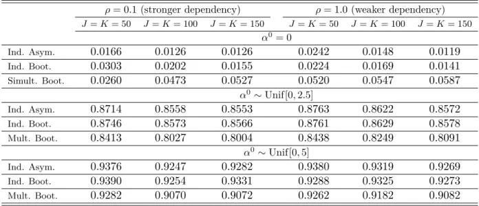
Our contribution lies in three aspects. First, we select the penalty level by controlling the aggregated errors in a system of high-dimensional sparse regressions, and we establish the bounds on the estimated coefficients. Furthermore, we show the implication of the restricted eigenvalue (RE) condition at a population level. Secondly, an easily implemented algorithm for effective estimation and inference is proposed. In fact, the offered estimation scheme al-lows us to make local and global inference on any set of parameters of interest. Thirdly, we run numerical experiments to illustrate good performance of our joint penalty relative to the single equation estimation, and we show the finite sample improvement of our multiplier block bootstrap procedure on the parameter inference. Finally, an application of textual sentiment
spillover effects on the stock returns in a financial market is presented.
In the literature, the fundamental results on achieving near oracle rate for penalizedℓ1-norm
estimators are developed by Bickel et al. (2009). There are many related articles on deriving near-oracle bounds using the ℓ1-norm penalization function for the i.i.d. case, such as
Bel-loni et al. (2011); BelBel-loni and Chernozhukov (2013). There are also many extensions to the LASSO estimation with dependent data. For example, Basu and Michailidis (2015) study the consistency of the estimator in sparse high-dimensional Gaussian time series models; Kock and Callot (2015) consider the high-dimensional near-oracle inequalities in large vector autoregres-sive (VAR) models; Lin and Michailidis (2017) look at the regularized estimation and testing for high-dimensional multi-block VAR models. However, the majority of the literature imposes a Gaussian or sub-Gaussian assumption on the error distribution; this is rather restrictive and excludes heavy tail distributions. For dependent data, Wu and Wu (2016) discuss the possibility of relaxing the sub-Gaussian assumption by generalizing Nagaev-type inequalities allowing for only moment assumptions. For the case of LASSO the analysis assumes the fixed design, which rules out the most important applications mentioned earlier in the introduction.
Theoretically, the LASSO tuning parameter selection requires characterizing the asymptotic distribution of the maximum of a high dimensional random vector. Chernozhukov et al. (2013) develop a Gaussian approximation for the maximum of a sum of high-dimensional random vectors, which is in fact the basic tool for modern high-dimensional estimation. Here it is applied to the LASSO inference. Moreover, Chernozhukov et al. (2019) deliver results for the case of β-mixing processes. Although it is quite common to assume a mixing condition which is at base a concept yielding asymptotic independence, it is not in general easy to verify the condition for a particular process, and some simple linear processes can be excluded from the strong mixing class, Andrews (1984). With an easily accessible dependency concept, Zhang and Wu (2017a) derive Gaussian approximation results for a wide class of stationary processes. Note that the dependence measure is linked to martingale decompositions and is therefore readily connected with a pool of results on tail probabilities, moment inequalities and central limit theorems of martingale theory. Our results are built on the above-mentioned theoretical works and we extend them substantially to fit into the estimation in a system of regression equations. In particular, our LASSO estimation is with random design for dependent data; therefore, we need to deal with the population implications of the Restricted Eigenvalue (RE) condition. Moreover, we show the interaction between the tail assumption and the dimensionality of the covariates in our theoretical results.
In the meantime, the issue of simultaneous inference is challenging and has motivated a series of research articles. For the case of i.i.d. data, Belloni et al. (2011, 2014), Zhang and Zhang (2014), Javanmard and Montanari (2014), van de Geer et al. (2014), Neykov et al. (2018), Chernozhukov et al. (2018), Zhu and Bradic (2018), among others, develop confidence intervals of low-dimensional variables in high-dimensional models with various forms of de-biased/orthogonalization methods. Still in the case of i.i.d. data, Belloni et al. (2015b) establish a uniform post-selection inference for the target parameters defined via de-biased Huber’s Z -estimators when the dimension of the parameters of interest is potentially larger than the sample size, where they employ the multiplier bootstrap to the estimated residuals. Wild and
residual bootstrap-assisted approaches are also studied in Dezeure et al. (2017); Zhang and Cheng (2017) for the case of mean regression. And more recently, Krampe et al. (2018) extend the approaches to test large groups of coefficients in sparse VAR models. We pick up the line of the inference analysis of Belloni et al. (2015b) and employ it in a temporal and cross-sectional dependence framework, thus making it applicable to a rich class of high-dimensional time series. This allows us to embed the high-dimensional VAR model as a special case. Our core proof strategy is different, as it is well known that the technique for handling the suprema of empirical processes indexed by functional classes with dependent data is not the same as in i.i.d. cases. For instance, the key Bahadur representation in Belloni et al. (2015b) applies maximal inequalities derived in Chernozhukov et al. (2014) for i.i.d. random variables, while we derive the key concentration inequalities based on a martingale approximation method.
Our proposed estimation framework is complement to the literature on model selection for Gaussian Graphical model (GGM) (see e.g. Yuan and Lin (2007)), which has a wide spectrum of applications in statistics. A GGM can be connected with LASSO regression for estimating sparse correlation networks, and therefore is equivalent to our context with a partial correla-tion network, Meinshausen et al. (2006). In particular, we may find an equacorrela-tion-by-equacorrela-tion relationship to the GGM, and we acknowledge that a similar framework with spatial temporal dependence can be developed. In addition, there is a big literature on social network analysis, which embeds the network information into a dynamic model in advance; see for example Zhu et al. (2017, 2019); Chen et al. (2019); Huang et al. (2016). Relatively, our approach is less structural as we treat the network structure to be unknown and uncover it using LASSO.
The following notations are adopted throughout this paper. For a vector v= (v1, . . . , vp)⊤,
let |v|∞ def= max16j6p|vj| and |v|s def= (Ppj=1|vj|s)1/s, s > 1. For a random variable X, let
kXkq def= (E|X|q)1/q, q > 0. For any function on a measurable space g : W → IR, En(g) def=
n−1Pnt=1{g(ωt)} and Gn(g)def= n−1/2Pnt=1[g(ωt)−E{g(ωt)}]. Given two sequences of positive
numbersan and bn, write an .bn if there exists constantC >0 (does not depend on n) such
thatan/bn6C. For a sequence of random variablesxn, we use the notationxn.Pbnto denote
xn=OP(bn). For any finitely discrete measureQ on a measurable space, letLq(Q) denote the
space of all measurable functionsf :Z →IR such thatkfkQ,q def= (Q|f|q)1/q <∞, where Qf def=
R
f dQ. For a class of measurable functionsF, theǫ-covering number with respect to theLq(Q
)-semimetric is denoted as N(ǫ,F,k · kQ,q), and let ent(ǫ,F) = log supQN(ǫkF¯kQ,q,F,k · kQ,q)
with ¯F = supf∈F|f| (the envelope) denote the uniform entropy number. It should be noted that we suppress the notation of the outer expectation E∗ to E and outer probability P∗ to P when measurability issues are encountered. Details may be found in the Chapter 1 of Van Der Vaart and Wellner (1996).
The rest of the article is organized as follows. Section 2 shows the system model with a few examples. Section 3 introduces the sparsity method for effective prediction and provides an algorithm for the joint penalty level of LASSO via bootstrap. In Section 4 we propose approaches to implementing individual and simultaneous inference on the coefficients. Main theorems are listed in Section 5. In Section 6 and 7 we deliver the simulation studies and an empirical application on textual sentiment spillover effects. The technical proofs and other details are given in the supplementary materials. The codes to implement the algorithms are
publicly accessible via the website www.quantlet.de.
2
The System Model
In this section, we present a general framework which covers many applications in statistics. Consider the system of regression equations (SRE):
Yj,t =Xj,t⊤βj0+εj,t, Eεj,tXj,t= 0, j= 1, ..., J, t= 1, . . . , n,
whereXj,t= (Xjk,t)Kk=1j . Without loss of generality, we assume the dimension of the covariates
is identical among all equations thereafter, namely Kj = dim(Xj,t) ≡K, for j = 1, . . . , J. We
allow the dimensionKofXj,tand the number of equations,Jto be large, potentially larger than
n, which creates an interplay with the tail assumptions on the error processesεj,t. Both spatial
and temporal dependency are allowed and we will obtain results on prediction and inference. The SRE framework is a system of regression equations, which includes the following im-portant special cases.
Example 1 (Many Regression Models). Suppose that we are interested in estimating the
predictive models for the response variables Um,t:
Um,t=Xt⊤γm0 +εm,t, Xt∈IRK, Eεm,tXt= 0, m= 1, . . . , M,
with auxiliary regressions to model predictive relations between covariates:
Xk,t=X−⊤k,tδk0+νk,t, Eνk,tX−k,t= 0, k= 1, . . . , K,
whereX−k,t= (Xℓ,t)ℓ=k6 ∈IRK−1, andδ0kis defined by the OLS estimator in population, namely
arg min
δk 1 n
Pn
t=1E(Xk,t−X−⊤k,tδk)2. This is a special SRE model with
(Yj,t, Xj,t, εj,t, β0j) = (Uj,t, Xt, εj,t, γj0), j= 1, . . . , M,
(Yj,t, Xj,t, εj,t, βj0) = (X(j−M),t, X−(j−M),t, ν(j−M),t, δ0(j−M)), j =M+ 1, . . . , J =M+K.
It can be seen that we only put contemporaneous exogeneity conditions for Xt. It is worth
mentioning that this SRE case is closely related to the semiparametric estimation framework studied in Section 2.4 in Belloni et al. (2015b). Here, the understanding of the predictive relations between covariates is important for constructing joint confidence intervals for the entire parameter vector {(γmk0 )Kk=1}M
m=1 in the main regression equations. Indeed, the construction
relies on the semi-parametrically efficient point estimators obtained from the empirical analog of the following orthogonalized moment equation:
E[(Umk,t0 −Xk,tγ0mk)νk,t] = 0, k= 1, . . . , K, m= 1, . . . , M, (2.1)
where U0
mk,t = Um,t −X−⊤k,tγm(0 −k) is the response variable minus the part explained by the
parameters replaced by the estimators.
Example 2(Simultaneous Equation Systems (SES)). Suppose there are many regression
equa-tions in the following form:
Um,t =U−⊤m,tδ0m+Xt⊤γm0 +εm,t, m= 1, . . . , M.
Move all the endogenous variables to the left-hand side and rewrite the model in the vector form
DUt=ΓXt+εt,
which is also called the structural form of the model. Suppose that D is invertible. Then the corresponding reduced form is given by
Ut=BXt+νt, Eνm,tXt= 0, m= 1, . . . , M, (2.2)
withB=D−1Γ and νt=D−1εt. In this case the Yj,t’s and Xj,t’s in SRE have no overlapping
variables. A high-dimensional SES can be considered as a special case of SRE with (Yj,t, Xj,t, εj,t, β0j) = (Uj,t, Xt, νj,t,B⊤j·), j= 1, . . . , M.
Example 3 (Large Vector Autoregression Models). In the case where the covariates involve
lagged variables of the response, SRE can be written as a large vector autoregression model. For example, the VAR(p) model,
Ut= p
X
ℓ=1
BℓUt−ℓ+εt, Eεm,tUt−ℓ= 0, m= 1, . . . , M, (2.3)
whereUt= (U1,t, U2,t, . . . , UM,t)⊤, andεtis anM-dimensional white noise or innovation process;
see e.g. Chapter 2.1 in Lütkepohl (2005). It is a special SRE case again with
(Yj,t, Xj,t, εj,t, βj0) = (Uj,t,(Ut⊤−1, . . . , Ut⊤−p)⊤, εj,t,(B1j·, . . . ,Bpj·)⊤), j = 1, . . . , M.
Such dynamics are of interest in biology to understand dynamic gene expression network association using micro array data; see for example Opgen-Rhein and Strimmer (2007); Ramirez et al. (2017); Dimitrakopoulou et al. (2011). It is understood that a crucial feature for many gene networks is their inherent sparsity. The issue of the number of variables involved is potentially larger than the sample size can be addressed by LASSO. Our methodology can help to analyze a gene interaction correlation network in a high dimensional regression scheme. In particular, suppose that each vertex represents a gene j collected at time point t with Uj,t as its gene
expression and an edge connects two genes if they are correlated.
3
Effective Prediction Using Sparsity Method
In this section, we present our model setup and the LASSO estimation algorithm, including the joint penalty selection procedure.
3.1 Sparsity in SRE
The general SRE structure makes it possible to predictYj,t using Xj,t effectively. Note that the
dimension ofXj,t is large, potentially larger thann. Without loss of generality we assume exact
sparsity of β0
j throughout the paper:
sj =|βj0|06s=O(n), j = 1, . . . J, (3.1)
where theℓ0-norm, | · |0, is the number of nonzero components of a vector.
Comment 3.1. It is now well understood that sparsity can be easily extended to approximate
sparsity, in which the sorted absolute values of coefficients decrease fast to zero. To be more specific, when βjk0 is not sparse, we shall define an intermediary optimal value for our true coefficients, i.e. βjk∗ . Let LCp def= min
|βj|06p
[En{Xj,t⊤(βj −βj0)}2]1/2, additionally with proper
conditions on the design matrix, the optimal sparsity level is given by s∗
j = min 06p6(K∧n)LC 2 p + ( max 16k6KΨ 2
jk)p/n, where Ψ2jk is the long run variance of √1n
Pn
t=1εj,tXjk,t. Then the oracle βjk∗
is defined to be arg min
|βj|06s∗j
En{Xj,t⊤(βj −βj0)}2. Thus an additional term involving LCs∗
j will
appear in the bound in case of the true signal βjk0 is not sparse. With approximate sparsity we mean that the true signal is not sparse but nevertheless can be approximated by an exact sparsity set-up well, namely |β0jk|6Ak−γ (ranked in descending order), where γ >0.5, and by takings∗
j ∝n1/(2γ) the goal would be achieved.
For this situation one employs anℓ1-penalized estimator of βj0 of the form:
b βj = arg min β∈IRK 1 n n X t=1 (Yj,t−Xj,t⊤β)2+ λ n K X k=1 |βk|Ψjk, (3.2)
where λ is the joint "optimal" penalty level and Ψjk’s are penalty loadings, which are defined
below in (3.3).
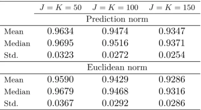
A first aim is to obtain performance bounds with respect to the prediction norm: |βbj−β0j|j,prdef= 1 n n X t=1 Xj,t⊤(βbj−β0j) 21/2 ,
where the outside j indicates to use the covariates in the jth equation Xj,t in computing the
prediction norm, and the Euclidean norm:
|βbj−βj0|2 def= K X k=1 (βbjk−βjk0 )2 1/2 .
To achieve good performance bounds, we first consider "ideal" choices (IC) of the penalty level and the penalty loadings. Let
Sjk = 1 √ n n X t=1 εj,tXjk,t,
where for a moment we assume to be able to observeεj,t =Yj,t−Xj,t⊤βj0. In practice one obtains
an approximation by stepwise LASSO. Set Ψjk def=
q
avar(Sjk), (3.3)
λ0(1−α)def= (1−α)−quantile of 2c√n max
16j6J,16k6K|Sjk/Ψjk|, (3.4)
where c > 1, e.g., c = 1.1, and 1−α is a confidence level, e.g. α = 0.1, where the long run variance is denoted by avar.
Theoretically, we can characterize the rate of λ0(1−α) by the tail probability of S jk (see
Theorem 5.1), also via Gaussian Approximation as in corollary 5.4. To calculateλ0(1−α) from data, we can also use a Gaussian approximation based on:
Q(1−α)def= (1−α)−quantile of 2c√n max
16j6J,16k6K|Zjk/Ψjk|,
where {Zjk} are multivariate Gaussian centered random variables with the same long run
co-variance structure as{Sjk}. Alternatively, we can employ a multiplier bootstrap procedure to
estimate IC empirically to achieve a better finite sample performance; see for example Cher-nozhukov et al. (2013). In case of dependent observations over time, it is understood that data cannot be resampled directly as in the the i.i.d. case, as the dependency structure of the under-lying processes will be lost. A usual solution to this problem is to consider a block bootstrap procedure, where the data are grouped into blocks, resampled and concatenated. In particular, we will adopt an estimate of IC by a multiplier block bootstrap procedure. The theoretical properties of LASSO and the tuning parameter choices are presented in Section 5.1-5.4.
3.2 Multiplier Bootstrap for the Joint Penalty Level
In this subsection, we introduce an algorithm to approximate the joint penalty level via a block multiplier bootstrap procedure, which is particularly non-overlapping block bootstrap (NBB). Consider the system of equations with dependent data:
Yj,t =Xj,t⊤βj0+εj,t, Eεj,tXj,t= 0, j= 1, ..., J, t= 1, . . . , n, (3.5)
S1 Run the initial ℓ1-penalized regression equation by equation, i.e. for thejth equation,
e βj = arg min β∈IRK 1 n n X t=1 (Yj,t−Xj,t⊤β)2+ λj n Kj X k=1 |βjk|Ψjk, (3.6)
where λj are the penalty levels and Ψjk are the penalty loadings. For instance, we
can take the X-independence choice using Gaussian approximation (in the heteroscedas-ticity case): 2c′√nΦ−1{1 − α′/(2K)} for λj, where Φ(·) denotes the cdf of N(0,1),
α′ = 0.1, c′ = 0.5, and choose qlvar(Xjk,tε˘j,t) for the penalty loadings, where ˘εj,t are
preliminary estimated errors and lvar(Xjk,tε˘j,t) is an estimate of the long-run variance
P∞
ℓ=−∞E(Xjk,tε˘j,tXjk,(t−ℓ)ε˘j,(t−ℓ)), e.g. the Newey-West estimator is given by pn
X
ℓ=−pn
k(ℓ/pn) cov(Xjk,tε˘j,t, Xjk,(t−ℓ)ε˘j,(t−ℓ)),
withk(z) = (1− |z|)1(|z|61). We note that theX-independent penalty (using Gaussian approximation) is more conservative, as the correlations among regressors can be adapted in theX-dependent case (using a multiplier bootstrap) with a less aggressive penalty level. S2 Obtain the residuals for each equation byq εej,t = Yj,t − Xj,t⊤βej, and compute Ψjk =
lvar(Xjk,tεej,t).
S3 Divide {ε˜j,t} into ln blocks containing the same number of observations bn, n = bnln,
where bn, ln ∈ Z. Then choose λ= 2c√nq(1[B]−α), where q(1[B]−α) is the (1−α) quantile of
max 16j6J,16k6K|Z [B] jk /Ψjk|, and Z [B] jk are defined as Zjk[B]= √1 n ln X i=1 ej,i ibn X l=(i−1)bn+1 ˜ εj,lXjk,l, (3.7)
ej,i are i.i.d. N(0,1) random variables independent of the data.
The bootstrap consistency regarding Zjk[B]is proved in Theorem 5.3.
Comment 3.2 (Block bootstrap procedures). (i) Concerning the determination of bn, we
shall report the prediction norm with several block sizes bn and select the one with the
best prediction performance in the simulation study. In addition, if it is the case that n
cannot be divided by bn with no remainder, one can simply take ln = ⌊n/bn⌋ and drop
the remaining observations.
(ii) Other forms of multiplier bootstrap with any random multipliers centered around 0 can also be considered.
(iii) Alternative block bootstrap procedures can be adopted, such as the circular bootstrap and the stationary bootstrap among others; see for example Lahiri et al. (1999) for an overview.
4
Valid Inference on the Coefficients
With a reasonable fitting of LASSO on hand, we can proceed to investigate the issue of simul-taneous inference. This section focuses on SRE of Example 2. We allow the covariates in each equation to be different.
The basic idea to facilitate inference is to formulate the estimation in a semi-parametric framework. With partialing out the effect of the nonparametric coefficient(s), we can achieve the desired estimation accuracy of the parametric component of interest. This trick is referred
to as "Neyman orthogonalization". Notably, the procedure is equivalent to the well known de-sparsification procedure in the mean square loss case, which is developed for the inference on the estimated zero coefficients by LASSO. It thus serves the same purpose of generating a (robust) de-sparsified estimation for LASSO inference.
We list three algorithms to estimate βjk0 . Algorithm 1 is easy to implement and algorithm 2 is tailored to the cases of heavy-tailed distribution of the error term, as Least Absolute Deviation (LAD) regression is well known to be robust against outliers. Algorithm 3 considers a double selection procedure aimed at remedying the bias due to omitted variables by one step selection, while also accounting for the cases of heteroscedastic errors.
Algorithm 1: LS-based algorithm
S1 Consider Yj,t =Xjk,tβ0jk+Xj(⊤−k),tβj(0−k)+εj,t, run (post) LS LASSO procedure (for each
j), and keep the quantityXj(⊤−k),tβbj([1]−k) for eachk.
S2 Run (post) LS LASSO (for each j, k) by regressingXjk,t=Xj(⊤−k),tγj(0−k)+vjk,t, and keep
the residuals as vbjk,t=Xjk,t−Xj(⊤−k),tγbj(−k).
S3 Run LS IV regression ofYj,t−Xj(⊤−k),tβbj([1]−k)onXjk,tusingvbjk,tas an instrument variable,
attaining the final estimatorβb[2]jk.
Algorithm 2: LAD-based algorithm
S1 and S2 are the same as Algorithm 1. S3′ Run LAD IV regression ofYj,t−X⊤
j(−k),tβb [1]
j(−k) onXjk,t usingvbjk,t as an instrument
vari-able, attaining the final estimator βbjk[2]. We refer to Belloni et al. (2015b); Chernozhukov and Hansen (2008) for more details about how to achieve the estimator in this step. The theoretical properties of the estimators βbj([1]−k) and γbj(−k) in S1 and S2 are provided in Corollary 5.1 or 5.4 (see Corollary A.1 or A.4 in the supplementary correspondingly if the joint penalty over equations is employed), and Theorem A.4 for post LASSO, respectively. The uniform Bahadur representation and the Central Limit Theorem of the estimatorβbjk[2] in S3 or S3′ are established in Theorem 5.4 and Corollary 5.6.
Comment 4.1. Our algorithms follow patterns discussed in Belloni et al. (2015b,a) in the i.i.d.
settings. The IV estimator obtained in S3 of Algorithm 1 reduced to the de-biased LASSO estimator (Zhang and Zhang, 2014; van de Geer et al., 2014) and is also first-order equivalent to the double LASSO method in Belloni et al. (2011, 2014). In particular, the estimator under LS IV regression (2-step least square regression) is given by
b βjk[2]= (vbjk⊤Xjk)−1vb⊤jk(Yj−Xj(⊤−k)βb [1] j(−k)) = (vbjk⊤Xjk)−1bv⊤jkYj− X m6=k b vjk⊤Xjm b v⊤ jkXjk b βjm[1]. (4.1)
The second line in (4.1) is exactly the same as the de-biased or de-sparsified LASSO estimator given in Eq. (5) in Zhang and Zhang (2014) or Eq. (5) in van de Geer et al. (2014). As remarked
in Belloni et al. (2015b,a), one can alternatively implement an algorithm via double selection as in Belloni et al. (2011, 2014). In particular, heteroscedastic LASSO is employed in S2′′ and the IV regression is replaced by a either LASSO or LAD regression on the target variable and all covariates selected in the first two steps.
Algorithm 3: Double selection-based algorithm
S1′′ Run LS LASSO (for eachj) ofYj,t on Xj,t:
b βj[1] = arg min β 1 n n X t=1 (Yj,t−Xj,t⊤β)2+ λ n|Ψbjβ|1.
S2′′ Run Heteroscedastic LASSO (for eachj, k) of Xjk,t onXj(−k),t:
b γj(−k)= arg min γ 1 n n X t=1 (Xjk,t−Xj(⊤−k),tγ)2+ λ′ n|Γbjγ|1,
where penalty loadings Γbj can be initialized as
q
lvar{Xjℓ,t(Xjk,t−n1 Pnt=1Xjk,t)} and
then refined by qlvar(Xjℓ,tvbjk,t), for ℓ 6= k, and vbjk,t = Xjk,t−Xj(⊤−k),tbγj(−k) can be
obtained by using the initial ones.
S3′′ Run LS regression ofYj,t on Xjk,t and the covariates selected in S1′′ and S2′′:
b βj[2] = arg min β { 1 n n X t=1
(Yj,t−Xj,t⊤β)2 : supp(β−k)⊆supp(βbj([1]−k))∪supp(bγj(−k))}.
S3′′′ Run LAD regression ofYj,t on Xjk,t and the covariates selected in S1′′ and S2′′:
b βj[2] = arg min β { 1 n n X t=1
|Yj,t−Xj,t⊤β|: supp(β−k)⊆supp(βbj([1]−k))∪supp(bγj(−k))}.
As shown in Belloni et al. (2011) and Belloni et al. (2015a), the double selection approach in S3′′ or S3′′′ creates an orthogonality condition with respect to the space spanned by the covariates
selected by both steps, and thus generates an orthogonal relation to any space spanned by a linear projection of the covariates, e.g. bvjk,t. Therefore, the inference on the parameters may
still be applied as in the framework of Algorithm 1 and 2. Therefore, one may still find the theoretical properties of estimators in S1′′, S2′′, S3′′ (S3′′′) in Section 5 according to the links mentioned above.
4.1 Confidence Interval for a Single Coefficient
We discuss an inference framework developed for a single coefficient obtained from the afore-mentioned algorithms.
Let ψjk(Zj,t, βjk, hjk) denote the score function, where Zj,t = (Yj,t, Xj,t⊤)⊤, hjk(Xj(−k),t) =
(X⊤
1(Yj,t 6 Xjk,tβjk +Xj(⊤−k),tβj(−k))}vjk,t, define ωjk def= E{(√1nPnt=1ψ0jk,t)2} = Pn−1 ℓ=−(n−1)(1− |ℓ| n) cov(ψ0jk,t, ψjk,(t0 −ℓ)) withψ0jk,t def = ψjk(Zj,t, βjk0 , h0jk), andφjk def= ∂E{ψjk(Zj,t,β,h0jk)} ∂β |β=β0 jk.
Suppose we are interested in testing H0 :βjk0 = 0. For this purpose we employ the uniform
Bahadur representation (Theorem 5.4) to construct the confidence interval via a multiplier bootstrap procedure. In particular, the distribution of the asymptotically pivotal statistics:
Tjk = √ n(βbjk[2]−β0 jk) b σjk , (4.2)
is approximated via its block multiplier bootstrap counterpart:
Tjk∗ = √1 n ln X i=1 ej,i ibn X l=(i−1)bn+1 b ζjk,l, (4.3)
whereζbjk,t are pre-estimators ofζjk,t=−φjk−1σjk−1ψ0jk,t such that
max
(j,k),(j′,k′)| Pln
i=1ηbj′k′,iηbjk,i−Pln
i=1ηj′k′,iηjk,i|=OP({log(JK)}−2), withηjk,idef= √1
n
Pibn
l=(i−1)bn+1ζjk,l
and ηbjk,i def= √1nPibl=(in −1)bn+1ζbjk,l,ej,i are independently drawn from N(0,1), ln and bn are the
numbers of blocks and block size, respectively. More discussion on how one can construct the consistent pre-estimators ζbjk,t is stated in the supplementary material; see Comment B.5.
Let σbjk be any consistent estimator of σjk. Then the confidence interval is given by
CIjk∗ (α) : [βbjk[2]−σbjkn−1/2q∗jk(1−α),βbjk[2]+σbjkn−1/2q∗jk(1−α)], (4.4)
whereq∗jk(1−α) is the (1−α) quantile of the bootstrapped distribution of |Tjk∗|.
Comment 4.2 (Asymptotic Normality of βbjk[2]). As shown in Corollary 5.5 we have the limit
distribution of βbjk[2]:
σjk−1n1/2(βbjk[2]−βjk0 )→L N(0,1), (4.5) whereσjk = (φ−jk2ωjk)1/2. Therefore, the two-sided 100(1−α) confidence interval by asymptotic
normality for β0
jk is given by
CIjk(α) : [βb[2]jk −σbjkn−1/2Φ−1(1−α/2),βbjk[2]+σbjkn−1/2Φ−1(1−α/2)]. (4.6)
Comment 4.3(Residual Multiplier Bootstrap). Alternative bootstrap procedures may be
con-sidered as well, e.g. the residual multiplier bootstrap procedure:
b
εj,t =Yj,t−Xj,t⊤βb [1] j ,
then divide {εbj,t}into ln blocks of size bn, wherebnln=n, and for each block i= 1, . . . , ln,
ε∗j,t = (εbj,t− 1 n n X t=1 b εj,t)ej,i, fort∈ {(i−1)bn+ 1, . . . , ibn}.
Define Y∗
j,t =Xj,t⊤βb [1]
j +ε∗j,t and compute the bootstrap counterpart as
Tjk∗ = √ n(βb∗ jk−βb [1] jk) b σ∗ jk ,
whereβb∗jk andσbjk∗ are estimated using the bootstrap sample{Yj,t∗, Xj,t}.
4.2 Joint Confidence Region for Simultaneous Inference
We now continue to extend the single coefficient inference to simultaneous inference on a set of coefficients. As shown in the practical examples in Section C.1, it is essential to conduct simultaneous inference on a group of parameters G. In this case, the null hypothesis is: H0 :
βjk0 = 0, ∀(j, k) ∈ G, and the alternative HA :βjk0 6= 0, for some (j, k) ∈ G, where the group
Gis a set of coefficients with cardinality |G|. Suppose for thej-th equation there arepj target
coefficients and the cardinality|G|=PJj=1pj. This can be understood as a multiple estimation
problem compared to Section 4.1. Without loss of generality, we can rearrange the order of the variables and rewrite the regression equation for eachj as (consider the LAD-based model here) Yj,t= pj X l=1 Xjl,tβjl0 + K X l=pj+1 Xjl,tβjl0 +εj,t, Fεj(0) = 1/2 (4.7)
One follows the algorithms to obtain βbjl(1 6 l 6 pj) for each j. Then the idea of
simul-taneous inference is very straightforward. We aggregate the statistics Tjk in (4.2) by taking
the maximum and minimum over the setG. Finally, the component-wise confidence interval is constructed with the quantiles of the bootstrap statistics over all bootstrap samples.
Denote q∗G(1−α) as the (1−α) quantile of max
(j,k)∈G|T ∗
jk|. A joint confidence region is then:
n β∈IR|G|: max (j,k)∈GTjk 6q ∗ G(1−α) and min (j,k)∈GTjk >−q ∗ G(1−α) o , (4.8)
and for each component (j, k)∈G, the confidence intervalCIf∗jk(α) is given by [βbjk[2]−σbjkn−1/2qG∗(1−
α),βbjk[2]+σbjkn−1/2q∗G(1−α)]. We show in Corollary 5.8 the consistency of this bootstrap
con-fidence band for simultaneous inference. Note that when there is only one parameter in G
for inference, the joint confidence region (4.8) will reduce to the single parameter confidence interval (4.4) as a special case.
5
Main Theorems
In this section, we present the theoretical foundations for the procedures given earlier. In particular, we discuss the properties of the theoretical choices of penalty level and the validity of the other two empirical choices, as well as the theoretical support for the simultaneous inference.
Throughout the whole section, we define Sjk def= n−1/2Pnt=1εj,tXjk,t, Sj· = (Sjk)Kk=1, and
Ψjk def=
q
{P∞ℓ=−∞E(Xjk,tXjk,(t−ℓ)εj,tεj,(t−ℓ))}1/2. Recall that for a single equation LASSO, we select the
penalty in the following ways:
a) theoretically, for each regression,λj isλ0j(1−α) (IC), i.e. the (1−α) quantile of
2c√n max
16k6K|Sjk/Ψjk| (note that this penalty takes into account the correlation among
regressors and is design adaptive);
b) an empirical choice given a Gaussian approximation result is Qj(1−α), which is defined
to be the (1−α) quantile of 2c max
16k6K
√
n|Zjk/Ψjk|, whereZjk’s are multivariate Gaussian
centered random variables with the same long run covariance structure as Sjk.
Alterna-tively, a canonical choice disregarding the correlation among regressors can be considered asQej(1−α)def= 2c√nΦ−1{1−α/(2K)}. We shall note that Qj(1−α) is not feasible but
can be estimated by simulations of Gaussian random variableZjk with estimated long run
variance covariance matrix. TypicallyQej(1−α) is more conservative thanQj(1−α).
c) another empirical choice of the penalty level is Λj(1−α) as the (1−α) quantile of
2c√n max
16k6K|Z [B]
jk /Ψbjk|(Zjk[B]’s are defined in (3.7)), and obtainable via the multiplier block
bootstrap technique.
5.1 Near Oracle Inequalities under IC
We first provide the near oracle inequalities for the single equation LASSO estimation ˜βj
ob-tained from (3.6) under the ideal choices (IC). For this purpose, a few assumptions and defini-tions are required.
(A1) For j = 1, . . . , J, k = 1, . . . , K, let Xjk,t and εj,t be stationary processes admitting the
following representation forms Xjk,t = gjk(Ft) = gjk(. . . , ξt−1, ξt) and εj,t = hj(Ft) =
hj(. . . , ηt−1, ηt), where ξt, ηt are i.i.d. random elements (innovations or shocks, allowing
for overlap; see Comment 5.1) across t, Ft = (. . . , ξt−1, ηt−1, ξt, ηt), gjk(·) and hj(·) are
measurable functions (filters). E(Xjk,tεj,t) = 0,for anyj, k∈1,· · ·, J,1,· · ·, K.
Definition 5.1. Let ξ0 be replaced by an i.i.d. copy of ξ0∗, andXjk,t∗ =gjk(. . . , ξ0∗, . . . , ξt−1, ξt).
Forq >1, define the functional dependence measure δq,j,k,t def= kXjk,t−Xjk,t∗ kq, which measures
the dependency of ξ0 onXjk,t. Also define ∆m,q,j,kdef= P∞t=mδq,j,k,t, which measures the
cumu-lative effect of ξ0 on Xjk,t>m. Moreover, we introduce the dependence adjusted norm of Xjk,t
as kXjk,·kq,ς def= supm>0(m+ 1)ς∆m,q,j,k(ς >0). Similarly, let η0 be replaced by an i.i.d. copy of
η∗
0, and ε∗j,t =hj(. . . , η0∗, . . . , ηt−1, ηt), we define kεj,·kq,ς def= supm>0(m+ 1)ς
P∞
t=mkεj,t−ε∗j,tkq
and kXjk,·εj,·kq,ς def= supm>0(m+ 1)ς
P∞
t=mkXjk,tεj,t−Xjk,t∗ ε∗j,tkq.
It should be noted that (A1) admits a wide class of processes. The largest value of ς which ensures a finite dependence adjusted norm characterizes the dependency structure of the process. The moment-based measure is directly connected with the impulse functions. A few examples for univariate time seriesZt are listed in Appendix C.2 in the supplementary materials.
(A2) Restricted eigenvalue (RE): given ¯c>1, forδ ∈IRK, with probability 1−O(1), κj(¯c)def= min |δT c j|16¯c|δTj|1, δ6=0 √s j|δ|j,pr |δTj|1 >0,
whereTj def= {k:βjk0 = 06 }and sj =|Tj|=O(n), δTjk=δk ifk∈Tj,δTjk= 0 if k /∈Tj.
(A3) kεj,·kq,ς <∞and kXjk,·kq,ς <∞(q>8).
Comment 5.1. We allow for overlap in the elements in ξt and ηt, as long as the
contempora-neous exogeneity condition E(Xjk,tεj,t) = 0 is satisfied. For example, consider the VAR(1)
model: Yt = AYt−1 +εt, with Yt, εt ∈ IRJ, and suppose that Yt admits the
representa-tion Yt = P∞l=0Alεt−l with εt−l as measurable functions of ξ−∞, . . . , ξt−l. Thus Xjk,t =
gjk(. . . , ξt−1) = P∞l=0[Al]kεt−1−l, where [Al]k is the kth row of the matrix Al, k = 1, . . . , J.
In this case no serial correlation in the innovationsεt’s would be sufficient forE(Xjk,tεj,t) = 0.
Comment 5.2. We show in Theorem B.2 (see the supplementary materials) that the RE
(A2) and RSE (A5) conditions can be implied by assumptions on the corresponding population variance-covariance matrix. This illustrates the feasibility of the RE/RSE assumption.
Lemma 5.1 (Prediction Performance Bound of Single Equation LASSO). Suppose (A1) and
(A2) (with ¯c = c+1c−1, c > 1), under the exact sparsity assumption (3.1) and given the event
λj >2c√n max
16k6K|Sjk/Ψjk|and another event which RE holds, then with probability 1−
O(1),β˜j
obtained from (3.6) satisfy
|β˜j−βj0|j,pr 6(1 + 1/c)
λj√sj
nκj(c)
max
16k6KΨjk. (5.1)
In addition, if (A2) (with 2¯c) holds, then with probability 1−O(1),
|β˜j−βj0|1 6
(1 + 2¯c)√sj
κj(2¯c) |
˜
βj −βj0|j,pr. (5.2)
Lemma 5.1 follows Theorem 1 of Belloni and Chernozhukov (2013). As the proof is built on inequalities and for the case of dependent data (A1) they remain unchanged, we omit the detailed proof here. To further characterize the rate of IC, we provide a tail probability for 2c√n max
16k6K|Sjk/Ψjk|under the moment assumption (A3). In particular, the rate depends on
the dependence adjusted norm kXjk,·εj,·kq,ς.
Theorem 5.1. Under (A1) and (A3), we have
P(2c√n max 16k6K|Sjk/Ψjk|>r)6C1̟nnr −qXK k=1 kXjk,·εj,·kqq,ς Ψqjk +C2 K X k=1 exp −C3r 2Ψ2 jk nkXjk,·εj,·k22,ς , (5.3)
where for ς >1/2−1/q (weak dependence case),̟n= 1; for ς <1/2−1/q (strong dependence
Comment 5.3. It can be seen in Theorem 5.1 that the rate of the dependence adjusted norm kXjk,·εj,·kq,ς plays an important role in the tail probability for 2c√n max
16k6K|Sjk/Ψjk|. Here we
discuss the rate under some special cases.
1. VAR(1)(Example 3, continued): Consider the VAR(1) model given byYt=AYt−1+εt,
where Yt, εt ∈ IRJ, and εt ∼ i.i.d. N(0,Σ). In this case Xjk,t = Yj,t−1 and K =J.
Sup-pose there exists a stationary representation of the model as Yt = P∞l=0Alεt−l. Then
we have kXjk,tεj,t −Xjk,t∗ ε∗j,tkq = kYj,t−1εj,t −Yj,t∗−1εj,tkq = k[At−1]j(ε0 −ε∗0)εj,tkq 6
2|[At−1]j|1µ2q, where µq def= maxjkεj,tkq and [At−1]j is the jth row of the matrix At−1.
Assume maxj|[At]j|1 6 |c|t with |c| < 1 (a geometric decay rate). It follows that
kXjk,·εj,·kq,ς = 2µ 2 q 1−|c|supm>0(m+ 1)ς P∞ t=m|c|t−1 6 (C/|c|)∨ {C(m∗ + 1)|c|m ∗ −1}, where
m∗ = (−ς/log|c| −1)∨0 and C > 0 depends on µq. Moreover, to justify the geometric
decay rate, we consider the example of Network Autoregressive (NAR) model as in Zhu et al. (2017) with A = ρW, where W is a row-normalized adjacency matrix which is pre-specified to indicate the social network connectedness andρ is the network parameter suggesting the strength of the network effects. In that case, assuming a geometric decay rate maxj|[At]j|1 6|c|t with|c|<1 again gives similar results.
2. Spatial autoregressive structure in εt: Consider the model Yj,t = Xj,t⊤βj + εj,t,
with εt = ρW εt+ηt, where W is a spatial weight matrix, ηt are i.i.d. and have
fi-nite qth moments µη q
def
= maxjkηj,tkq. For simplicity, here we assume Xj,t and εj,t
are independent. Suppose there exists a stationary representation of the error pro-cess given by εt = P∞l=0ρlWlηt−l. Then we have kXjk,tεj,t −Xjk,t∗ εj,t∗ kq 6 k(Xjk,t −
X∗
jk,t)εj,tkq+kXjk,t(εj,t−ε∗j,t)kq6kXjk,t−Xjk,t∗ kqkεj,tkq+kXjk,tkqk[ρtWt]j(η0−η∗0)kq6
|[(I−ρW)−1]j|1µηqkXjk,t−Xjk,t∗ kq+ 2|[ρtWt]j|1µηqkXjk,tkq. Assume maxj|[ρtWt]j|1 6|c|t
with|c|<1. It follows thatkXjk,·εj,·kq,ς 6C1kXjk,·kq,ς +C2supm>0(m+ 1)ς
P∞
t=m|c|t6
C1kXjk,·kq,ς +C3(m∗ + 1)|c|m
∗
−1, where m∗ = (−ς/log|c| −1)∨0 and C1, C2, C3 > 0
depend onµηq and kXjk,tkq.
3. General linear processes: To study more general spatial and temporal dependency,
consider the model Yj,t = Xj,t⊤βj +εj,t, with εt = P∞l=0Alηt−l. Again ηt are i.i.d. and
have finite qth moments µη q
def
= maxjkηj,tkq. If all the Al are diagonal matrices, there
is just temporal dependence, and if Al = 0 for l > 1 there exists only spatial depen-dence. Let atjk def= [At]jk be the element on the jth row and kth column of At.
As-sume P∞t=0Pk|at
jk| < ∞, Xj,t and εj,t to be independent. We have kXjk,·εj,·kq,ς 6
C1kXjk,·kq,ς +C2supm>0(m+ 1)ς
P∞
t=m
P
k|atjk|, where C1, C2 > 0 depend on µηq and
kXjk,tkq. Moreover, we have kmaxjk(Xjk,·εj,·)kq,ς 6 kmaxjkXjk,·kq,ςkmaxjεj,·kq,ς, and
particularly k|εt|∞kq 6 kmaxjPkatjk(ηk,0−ηk,0∗ )kq . qkmaxkmaxjajkt (ηk,0−ηk,0∗ )kq+
√ qlogJ{Pkmaxj(atjk)2(µ η 2)2}1/2 . q P kmaxj|atjk|µηq ∨ √ qlogJ{Pkmaxj(atjk)2}1/2µ η 2,
where the Rosenthal-Burkholder inequality is applied. Suppose thatP∞t=m(Pkmaxj|atjk|).
J(m∨1)−c, for some constant c > 0. If ς < c, we have kmax
jεj,·kq,ς 6C3supm>1(m+
1)ς(m∨1)−cJ√logJ 6C3supm>1(m+ 1)ς−cJ
√
logJ, whereC3>0 depends on µηq.
To summarize, if theqth moments are bounded by constant, the dependence adjusted norm kXjk,·εj,·kq,ς is also bounded in the first two examples where a geometric decay rate on the
coefficients is assumed; while in the case of general linear processes, it would depend on the rate of P∞t=0Pk|atjk|. In particular, suppose P∞t=mPk|atjk| .(m∨1)−c for c > 0. If c > ς, kXjk,·εj,·kq,ς is bounded (assume kXjk,·kq,ς is bounded).
Under the choice (IC) λ0j(1−α) is given by the (1−α) quantile of 2c√n max
16k6K|Sjk/Ψjk|,
combining the results of Lemma 5.1 and Theorem 5.1 we can get the bounds forλ0j(1−α) and further obtain the oracle inequalities as in Corollary 5.1.
Corollary 5.1 (Bounds for λ0
j(1−α) and Oracle Inequalities under IC). Under (A1)-(A3),
given λ0j(1−α) satisfying λ0j(1−α). max 16k6K kXjk,·εj,·k2,ς q nlog(K/α)∨ kXjk,·εj,·kq,ς(n̟nK/α)1/q , (5.4)
and the exact sparsity assumption (3.1), then β˜j obtained from (3.6)under IC satisfies
|β˜j−βj0|j,pr. √s j κj(¯c) max 16k6KΨjk kXjk,·εj,·k2,ς q log(K/α)/n∨ kXjk,·εj,·kq,ςn1/q−1(̟nK/α)1/q , (5.5)
with probability 1−α−O(1), where for ς > 1/2−1/q (weak dependence case), ̟n = 1; for
ς <1/2−1/q (strong dependence case), ̟n=nq/2−1−ςq.
Comment 5.4. The Nagaev type of inequality in (5.3) has two terms, namely an exponential
term and a polynomial term. It should be noted that if the polynomial term dominates, the above bound does not allow for ultra high dimension of K. Basically, we only allow for a polynomial rate K =O(nc˜), and the rate ofK interplays with the dependence adjusted norm kXjk,·εj,·kq,ς. In particular, to make sure that the estimators are consistent (i.e. the error
bounds tend to zero for sufficiently largen), for example, we need ˜c < q−1−υq/2−dq, if there existsq to guaranteekXjk,·εj,·kq,ς =O(nd) and 0< υ <1 such thatsj =O(nυ).
We now discuss the case of sub-Gaussian tail or sub-exponential tail, which is mostly assumed in the literature.
Comment 5.5. Suppose that a stronger exponential moment condition is satisfied,
kXjk,·εj,·kψν,ς = sup q>2
q−νkXjk,·εj,·kq,ς <∞, (5.6)
where kXjk,·εj,·kψν,ς is interpreted as the dependence adjusted sub-exponential (ν = 2) or
sub-Gaussian (ν = 1) norm. Consider the special case of VAR(1). As shown above, we have kXjk,tεj,t−Xjk,t∗ ε∗j,tkq 62|[At−1]j|1µ2q. In particular, it is known thatµq.qfor sub-exponential
variables and µq . √q for sub-Gaussian variables. Let ν = 2 and ν = 1 for the two cases
respectively, kXjk,·εj,·kψν,ς . (m∗+ 1)|c|m
∗
−1. Then applying the exponential tail bounds as
in Lemma B.4 in the supplementary material, we arrive at the following error bounds with probability 1−α−O(1), |β˜j−βj0|j,pr . √s j κj(¯c) max 16k6KΨjkkXjk,·εj,·kψν,0 {log(K/α)}1/γ √ n , γ = 2/(2ν+ 1), (5.7)
as λ0
j(1−α) .
√
n(logK)1/γ max
16k6KkXjk,·εj,·kψν,0. The bound (5.7) works with ultra-high
di-mensional rate exp(nrγ) (r <1) of K as only the exponential term shows in the inequality. In particular, supposesj =O(nυ), andkXjk,·εj,·kψν,0 =O(n
d), thenr+d+υ/2<1/2 is required
to ensure the consistency.
In the special case with i.i.d. data, the dependence adjusted norm would be kXjk,·εj,·kq,ς 6
2kXjk,tεj,tkq, and kXjk,·εj,·kψν,0 will be bounded by a constant which is relevant to the
corre-sponding tail assumptions of the moments. Compared to the standard rate for LASSO estima-tors such as in Theorem 1 of Belloni and Chernozhukov (2013) with independent errors, our results will be the same for the case of Gaussian innovation (i.e. ν = 0). Moreover, for time series data, disregarding the dependency adjusted norm term, our convergence rate of predic-tion norm qsjlogK/n (given ν = 0) is also of the same order as the rate for stable Gaussian
processes studied in Basu and Michailidis (2015).
5.2 Gaussian Approximation for Dependent Data
Now we look at the validity of the choice ofQj(1−α), which relies on a Gaussian approximation
theorem. First we define the Kolmogorov distance between any two K-dim random vectors.
Definition 5.2. Let X = (X1,· · ·, XK)⊤∈IRK, Y = (Y1,· · · , YK)⊤ ∈IRK. The Kolmogorov
distance between X andY is defined as
ρ(X,Y) = sup r>0 P(|X|∞>r)−P(|Y|∞>r) .
For each single equation j, aggregate the dependence adjusted norm overk= 1, . . . , K: k|Xj,·|∞kq,ς def= sup m>0 (m+ 1)ς ∞ X t=m δq,j,t, δq,j,tdef= k|Xj,t−Xj,t∗ |∞kq, (5.8)
whereq >1 andς >0. Moreover, define the following quantities
Φj,q,ς def= 2 max 16k6KkXjk,·kq,ςkεj,·kq,ς, Γj,q,ς def = 2kεj,·kq,ς XK k=1 kXjk,·kq/2q,ς 2/q Θj,q,ς def= Γj,q,ς∧ 2k|Xj,·|∞kq,ςkεj,·kq,ς(logK)3/2 . (5.9)
It is worth noting that the normk|Xj,·|∞kq,ς is a kind of aggregated dependence adjusted norm
for a vector of processes in comparison to the dependence adjusted norm for a univariate process as in Definition 5.1.
Some additional assumptions are required. Define L1,j = {Φj,4,ςΦj,4,0(logK)2}1/ς, W1,j =
(Φ6j,6,0+Φ4j,8,0){log(Kn)}7,W2,j= Φ2j,4,ς{log(Kn)}4,W3,j= [n−ς{log(Kn)}3/2Θj,2q,ς]1/(1/2−ς−1/q),
N1,j= (n/logK)q/2Θqj,2q,ς,N2,j=n(logK)−2Φj,4,ς−2 ,N3,j ={n1/2(logK)−1/2Θ−j,2q,ς1 }1/(1/2−ς).
(A4) i) (weak dependency case) Given Θj,2q,ς <∞with q>4 and ς >1/2−1/q, then
Θj,2q,ςn1/q−1/2{log(Kn)}3/2→0 and L1,jmax(W1,j, W2,j) =O(1) min(N1,j, N2,j).
ii) (strong dependency case) Given 0< ς <1/2−1/q, then Θj,2q,ς(logK)1/2 =O(nς) and
The assumptions impose mild restrictions on the dependency structure of covariates and error terms. They include a wide class of potential correlation and heterogeneity (including conditional heteroscedasticity), with possible allowance of the lagged dependent variables. Two examples of large VAR and ARCH for high-dimensional time series can be found in Appendix C.2 in the supplementary materials.
Comment 5.6 (Admissible Dimension Rates by the Conditions for Gaussian Approximation).
As discussed in Zhang and Wu (2017a), consider the case with Θj,2q,ς =O(K1/q) and Φj,2q,ς =
O(1), whereς >1/2−1/q. Then Θj,2q,ςn1/q−1/2{log(Kn)}3/2→0 becomes K{log(nK)}3q/2=
O(nq/2−1), which implies that L1,jmax(W1,j, W2,j) = O(1) min(N1,j, N2,j). This means with
(A4), the dimension K has to satisfy the condition K(logK)3q/2 =O(nq/2−1).
Theorem 5.2(Gaussian Approximation Results for Dependent Data). Under (A1) and
(A3)-(A4), for eachj= 1, . . . , J assume that there exists a constantcj >0such that min
16k6Kavar(Sjk)>
cj, then we have
ρ Dj−1Sj·, D−j1Zj→0, as n→ ∞, (5.10)
where Zj ∼N(0,Σj), Σj is the K×K long-run variance-covariance matrix of Xj,tεj,t, and Dj
is a diagonal matrix with the square root of the diagonal elements of Σj, namely
X∞
ℓ=−∞
E(Xjk,tXjk,(t−ℓ)εj,tεj,(t−ℓ))
1/2
=qavar(Sjk), for k= 1, . . . , K.
Comment 5.7. The conclusion in Theorem 5.2 can be held with stronger tail assumptions,
following Theorem 5.2 in Zhang and Wu (2017a).
Theorem 5.2 justifies the choice ofλj and ˜Qj(1−α), which leads to the following corollary:
Corollary 5.2. Under the conditions of Theorem 5.2, for each j we have
sup α∈(0,1) P{ max 16k6K2c √ n|Sjk/Ψjk|>Qj(1−α)} −α →0, as n→ ∞. (5.11)
It is worth noting that in practice the variance involved in the Gaussian approximation in 5.2 is not known; we shall discuss how we estimate the variance and also the validity of the Gaussian approximation result with an estimated variance. Given the realization Xj,1εj,1, . . . , Xj,nεj,n,
we propose to estimate the K×K long-run variance-covariance matrix Σj forj = 1, . . . , J as
follows, givenEXj,tεj,t= 0, and consider:
b Σj = 1 bnln ln X i=1 ibn X l=(i−1)bn+1 Xj,lεj,l Xibn l=(i−1)bn+1 Xj,lεj,l ⊤ . (5.12)
Moreover, the following corollary ensures that the Gaussian approximation results still hold if we use the estimate in (5.12).
Corollary 5.3. Let the conditions of Theorem 5.2 hold, and assume Φj,2q,ς <∞ with q > 4,
bn = O(nη) for some 0 < η < 1. Let Fς = n, for ς > 1 −2/q; Fς = lnbq/2n −ςq/2, for