B ayesian netw orks for classification, clustering, and high-
dim ensional data visualisation
A thesis
submitted to Cardiff University for the degree of
Doctor of Philosophy by
Gonzalo Andres Ruz Heredia
Manufacturing Engineering Centre Cardiff Uni versity
United Kingdom
UMI Number: U585111
All rights reserved
INFORMATION TO ALL USERS
The quality of this reproduction is dependent upon the quality of the copy submitted. In the unlikely event that the author did not send a complete manuscript and there are missing pages, these will be noted. Also, if material had to be removed,
a note will indicate the deletion.
Dissertation Publishing
UMI U585111
Published by ProQuest LLC 2013. Copyright in the Dissertation held by the Author. Microform Edition © ProQuest LLC.
All rights reserved. This work is protected against unauthorized copying under Title 17, United States Code.
ProQuest LLC
789 East Eisenhower Parkway P.O. Box 1346
SUMMARY
This thesis presents new developments for a particular class o f Bayesian networks which are limited in the number o f parent nodes that each node in the network can have. This restriction yields structures which have low complexity (number o f edges), thus enabling the formulation o f optimal learning algorithms for Bayesian networks from data. The new developments are focused on three topics: classification, clustering, and high-dimensional data visualisation (topographic map formation).
For classification purposes, a new learning algorithm for Bayesian networks is introduced which generates simple Bayesian network classifiers. This approach creates a completely new class o f networks which previously was limited mostly to two well known models, the naive Bayesian (NB) classifier and the Tree Augmented Saive Bayes (TAN) classifier. The proposed learning algorithm enhances the NB model by adding a Bayesian monitoring system. Therefore, the complexity o f the resulting network is determined according to the input data yielding structures which model the data distribution in a more realistic way which improves the classification performance.
Research on Bayesian networks for clustering has not been as popular as for classification tasks. A new unsupervised learning algorithm for three types o f Bayesian network classifiers, which enables them to carry out clustering tasks, is introduced. The resulting models can perform cluster assignments in a probabilistic way using the posterior probability o f a data point belonging to one o f the clusters. A
key characteristic o f the proposed clustering models, which traditional clustering techniques do not have, is the ability to show the probabilistic dependencies amongst the variables for each cluster. This feature enables a better understanding o f each cluster.
The final part o f this thesis introduces one o f the first developments for Bayesian networks to perform topographic mapping. A new unsupervised learning algorithm for the NB model is presented which enables the projection o f high-dimensional data into a two-dimensional space for visualisation purposes. The Bayesian network formalism o f the model allows the learning algorithm to generate a density model o f the input data and the presence o f a cost function to monitor the convergence during the training process. These important features are limitations which other mapping techniques have and which have been overcome in this research.
ACKNOWLEDGEMENTS
I would like to express my sincere gratitude to my supervisor Professor D.T. Pham for his excellent guidance throughout my research, as well as his practical and positive thinking which was very useful during the more difficult stages o f my research.
I would also like to thank my family for the support and encouragement they have given me always, and my wonderful girlfriend Pam for her support and unconditional love.
Special thanks to my friend Pedro Ortega who introduced me to the field o f Bayesian networks several years ago and with whom I have always been able to have fruitful discussion regarding my work.
Thank you to the members o f the MEC Machine Learning Group for providing interesting comments and presentations in our weekly meetings.
Thank you to the people in the computer lab where I work, for making it a cheerful place to study, as well as everyone at the MEC.
DECLARATION AND STATEMENTS
DECLARATION
This work has not previously been accepted in substance for any degree and is not concurrently submitted in candidature for any degree.
Signed ... (Gonzalo A. Ruz Heredia) Date 29/05/2008
STATEMENT 1
This thesis is being submitted in partial fulfillment o f the requirements for the degree of Doctor o f Philosophy (PhD).
Signed .. ... (Gonzalo A. Ruz Heredia) Date 29/05/2008
STATEMENT 2
This thesis is the result o f my own independent work/investigation, except where otherwise stated. Other sources are acknowledged by explicit references.
Signed (Gonzalo A. Ruz Heredia) Date 29/05/2008
STATEMENT 3
I hereby give consent for my thesis, if accepted, to be available for photocopying and for inter-library loan, and for the title and summary to be made available to outside organisations.
TABLE OF CONTENTS
SUM M ARY... I
ACKNOW LEDGEM ENTS...IV
DECLARATION AND STA T EM E N TS... V
TABLE OF C O N T E N T S... VI
LIST OF FIG U R ES... IX
LIST OF T A B L E S... XIV LIST OF SY M B O L S... XV ABBREVIATIONS... XVII 1 INTRODUCTION... 1 1.1 Mo t i v a t i o n...1 1.2 Aim a n d Ob j e c t i v e s...3 1.3 Me t h o d s...4 1.4 Ou t l in e o ft h e t h e s i s...5 2 BACKGROUND...8 2.1 Ra n d o m v a r i a b l e s a n d c o n d it io n a l i n d e p e n d e n c e...8 2 .2 Gr a p h t h e o r y...9 2.3 The Ma r k o v Co n d i t i o n... 10 2 .4 Ba y e s i a n n e t w o r k s... 11 2 .5 Le a r n i n g Ba y e s i a nn e t w o r k s...12 2 .6 Re c e n t Ba y e s i a n n e t w o r ka p p l i c a t i o n s... 14
2.7 Su m m a r y... 30
3 SIMPLE BAYESIAN NETWORK CLASSIFIERS...31
3.1 Pr e l i m i n a r i e s...31 3 .2 Ba y e s i a nn e t w o r k c l a s s i f i e r s...3 4 3.3 Tr a in in g s im p l e Ba y e s i a n n e t w o r k c l a s s i f i e r s... 3 8 3.3.1 N e tw o r k e n c o d in g ... 3 8 3 .3 .2 C o m p le x ity m e a s u r e ... 41 3 .3 .3 S im p le le a r n in g a lg o r ith m ...43 3 .4 Me t h o d s... 51 3 .5 Ex p e r im e n t a lr e s u l t s... 55 3 .6 Su m m a r y... 63
4 UNSUPERVISED TRAINING OF BAYESIAN NETW O RK S... 66
4.1 Pr e l i m i n a r i e s... 6 6 4 .2 Pr o b a b il is t ic c l a s s i f i e r s...7 0 4 .3 Cl a s s if ic a t io n E M a l g o r i t h m...7 9 4 .4 Pr o p o s e d u n s u p e r v i s e d t r a in in g a p p r o a c h...81
4 .4 .1 U n s u p e r v is e d tra in in g for C L m u ltin e ts c l a s s i f i e r ... 82
4 .4 .2 U n s u p e r v is e d tr a in in g fo r th e T A N c l a s s i f i e r ... 85 4 .4 .3 U n s u p e r v is e d tr a in in g fo r th e S B N c l a s s i f i e r ... 8 6 4 .5 Me t h o d s... 91 4 .5 .1 B en ch m a rk d ata s e t s ... 91 4 .5 .2 W o o d d e fe c t c la s s if ic a t io n ... 94 4 .5 .3 I n it ia lis a t io n ... 95 4 .6 Ex p e r im e n t a l r e s u l t s a n d d i s c u s s i o n s...95
4.7 S u m m a r y 101
5 TRAINING NAIVE BAYES MODELS FOR DATA VISUALISATION 102
5.1 Pr e l i m i n a r i e s...102
5.2 Na i v e Ba y e s m o d e l s...105
5.3 Tr a in i n g o fn a i v e Ba y e s m o d e l s f o r t o p o g r a p h ic m a p f o r m a t i o n.. 108
5.4 Si m u l a t i o n s...112
5.4.1 Map formation exam ple...112
5 .4 .2 Monitoring convergence...117
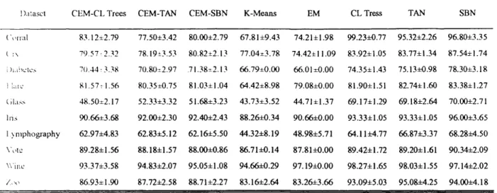
5 .4 .3 Comparing map quality with other techniques...124
5 .4 .4 Industrial application...167 5.5 Re l a t io n s w it h o t h e ra l g o r i t h m s...173 5.6 Su m m a r y... 174 6 C O NCLUSIO N... 176 6.1 Co n t r i b u t i o n s... 176 6 .2 Co n c l u s i o n s...177 6.3 Su g g e s t i o n s f o r f u t u r e r e s e a r c h... 179 REFERENCES... 181
LIST OF FIGURES
Figure 3.1 Naive Bayes classifier... 37
Figure 3.2 TAN classifier... 37
Figure 3.3 An example o f a Bayesian network with 3 nodes and 2 edges...40
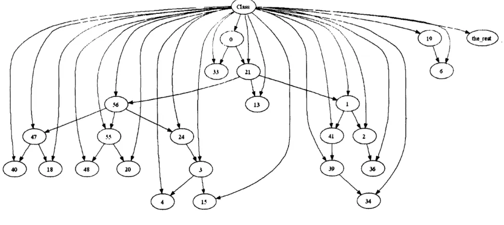
Figure 3.4 Naive Bayes model for the “Cleve” data set obtained by the SBN classifier when 10% o f the instances are used for training... 57
Figure 3.5 TAN model for the “Cleve” data set obtained by SBN classifier when 80% o f the instances are used for training... 58
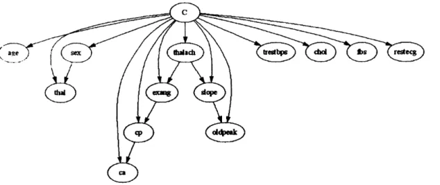
Figure 3.6 Network structure for the “Cleve” data set obtained by the SBN classifier when 50% o f the instances are used for training... 59
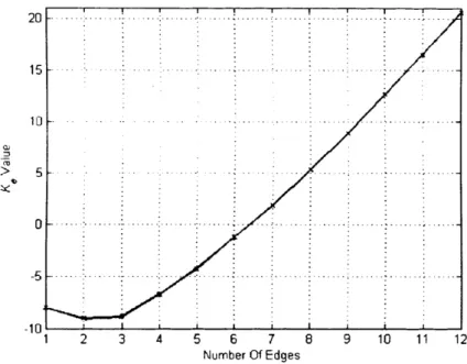
Figure 3.7 Plot illustrating the Ke values for each edge added during the Build Network procedure for the “Cleve” data set, when 50% o f the instances for training are used...60
Figure 3.8 The simple Bayesian network classifier for the control chart d a ta ...61
Figure 4.1 Bayesian network representation o f the naive Bayes classifier... 71
Figure 4.2 Chow & Liu’s tree algorithm ... 76
Figure 4.3 CL multinet classifier representation... 76
Figure 4.4 TAN learning process... 77
Figure 4.5 TAN classifier representation... 77
Figure 4.6 SBN classifier learning procedure...78
Figure 4.7 SBN classifier representation... 78
Figure 4.8 Unsupervised training o f CL trees...88
Figure 4.11 CL trees o f the “Corral” data s e t ...100
Figure 4.12 TAN o f the “Corral” data se t... 100
Figure 4.13 SBN o f the “Corral” data s e t... 100
Figure 5.1 Naive Bayes m odel...107
Figure 5.2(a) Naive Bayes map formation at / = 0...114
Figure 5.2(b) Naive Bayes map formation at t = 500... 114
Figure 5.2(c) Naive Bayes map formation at t — 1000... 115
Figure 5.2(d) Naive Bayes map formation at t = 5000... 115
Figure 5.2(e) Naive Bayes map formation at t = 10000... 116
Figure 5.2(f) Naive Bayes map formation at t = 100000... 116
Figure 5.3(a) Output o f example 1... 120
Figure 5.3(b) Output o f example 2 ... 120
Figure 5.3(c) Output o f example 3 ... 121
Figure 5.3(d) Log-likelihood convergence for the three examples... 121
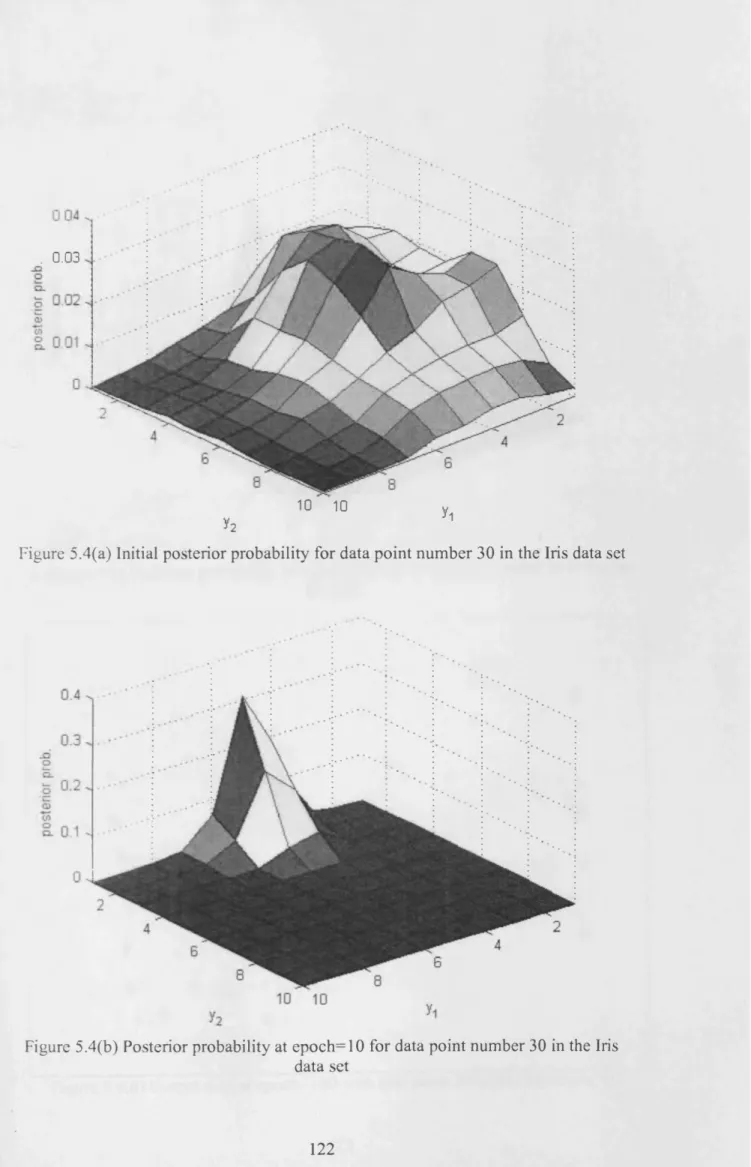
Figure 5.4(a) Initial posterior probability for data point number 30 in the Iris data set 122 Figure 5.4(b) Posterior probability at epoch=10 for data point number 30 in the Iris data s e t ...122
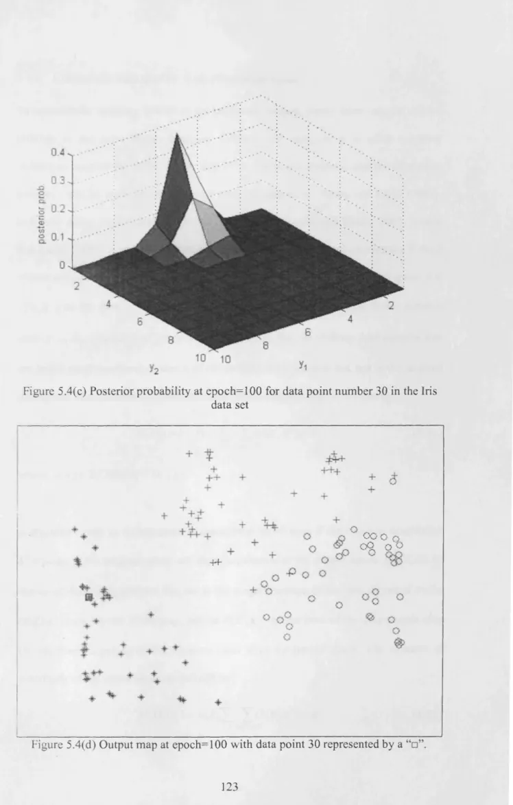
Figure 5.4(c) Posterior probability at epoch=100 for data point number 30 in the Iris data s e t ...123
Figure 5 .4(d) Output map at epoch=100 with data point 30 represented by a “ □ ” . ... 123
Figure 5.5(a) Australian data set projection using P C A ... 127
Figure 5.5(b) Australian data set projection using S O M ... 127
Figure 5.5(d) Australian data set projection using N B M ... 128
Figure 5.5(e) Trustworthiness measure for the Australian data set projection... 129
Figure 5.5(0 Continuity measure for the Australian data set projection...129
Figure 5.6(a) Breast data set projection using PC A ...131
Figure 5.6(b) Breast data set projection using SOM ...131
Figure 5.6(c) Breast data set projection using GTM ...132
Figure 5.6(d) Breast data set projection using N B M ...132
Figure 5.6(e) Trustworthiness measure for the Breast data set projection... 133
Figure 5.6(0 Continuity measure for the Breast data set projection... 133
Figure 5.7(a) Cleve data set projection using PCA... 135
Figure 5.7(b) Cleve data set projection using S O M ... 135
Figure 5.7(c) Cleve data set projection using G T M ... 136
Figure 5.7(d) Cleve data set projection using N B M ...136
Figure 5.7(e) Trustworthiness measure for the Cleve data set projection...137
Figure 5.7(0 Continuity measure for the Cleve data set projection... 137
Figure 5.8(a) Crx data set projection using P C A ... 139
Figure 5.8(b) Crx data set projection using SO M ... 139
Figure 5.8(c) Crx data set projection using G T M ... 140
Figure 5.8(d) Crx data set projection using N B M ... 140
Figure 5.8(e) Trustworthiness measure for the Crx data set projection... 141
Figure 5.8(0 Continuity measure for the Crx data set projection... 141
Figure 5.9(a) Diabetes data set projection using P C A ... 143
Figure 5.9(b) Diabetes data set projection using SO M ... 143
Figure 5.9(c) Diabetes data set projection using G T M ... 144
Figure 5.9(e) Trustworthiness measure for the Diabetes data set projection... 145
Figure 5.9(f) Continuity measure for the Diabetes data set projection... 145
Figure 5 .10(a) Heart data set projection using P C A ...147
Figure 5 .10(b) Heart data set projection using S O M ... 147
Figure 5 .10(c) Heart data set projection using G T M ... 148
Figure 5.10(d) Heart data set projection using N B M ... 148
Figure 5 .10(e) Trustworthiness measure for the Heart data set projection...149
Figure 5 .10(f) Continuity measure for the Heart data set projection... 149
Figure 5 .1 1(a) Ionosphere data set projection using P C A ... 151
Figure 5.11 (b) Ionosphere data set projection using SO M ... 151
Figure 5 .1 1(c) Ionosphere data set projection using G T M ... 152
Figure 5 .1 1(d) Ionosphere data set projection using N BM ...152
Figure 5 .1 1(e) Trustworthiness measure for the Ionosphere data set projection 153 Figure 5.11(f) Continuity measure for the Ionosphere data set projection...153
Figure 5.12(a) Iris data set projection using PCA... 155
Figure 5 .12(b) Iris data set projection using S O M ... 155
Figure 5.12(c) Iris data set projection using G T M ...156
Figure 5 .12(d) Iris data set projection using N B M ... 156
Figure 5 .12(e) Trustworthiness measure for the Iris data set projection...157
Figure 5 .12(f) Continuity measure for the Iris data set projection...157
Figure 5 .13(a) Pima data set projection using PC A ...159
Figure 5 .13(b) Pima data set projection using SOM ...159
f igure 5.13(c) Pima data set projection using GTM ...160
Figure 5.13(d) Pima data set projection using N B M ...160
Figure 5.13(f) Continuity measure for the Pima data set projection... 161
Figure 5 .14(a) Wine data set projection using P C A ...164
Figure 5 .14(b) Wine data set projection using S O M ... 164
Figure 5.14(c) Wine data set projection using G T M ... 165
Figure 5 .14(d) Wine data set projection using N B M ... 165
Figure 5 .14(e) Trustworthiness measure for the Wine data set projection... 166
Figure 5.14(0 Continuity measure for the Wine data set projection... 166
Figure 5.15(a) Wood data set projection using P C A ...170
Figure 5 .15(b) Wood data set projection using SO M ...170
Figure 5.15(c) Wood data set projection using G T M ...171
Figure 5.15(d) Wood data set projection using N B M ...171
Figure 5.15(e) Trustworthiness measure for the Wood data set projection... 172
LIST OF TABLES
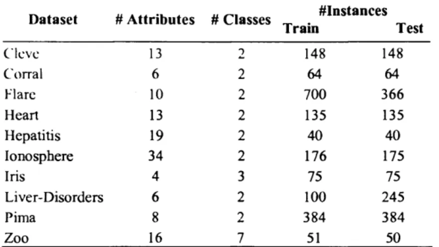
Tabic 3.1 Description o f the data sets used in the first experim ent... 54
Table 3.2 Comparison o f the NB, TAN, and the SBN on the test sets...62
Table 3.3 Classification accuracy on the control chart pattern recognition problem ..62
Table 4.1 Description o f the benchmark data s e ts ...93
Table 4.2 Experimental results using the benchmark data s e ts ...99
Table 4.3 Experimental results using the wood data se t... 99
LIST OF SYMBOLS
The i-th attribute. A set o f attributes. Probability distribution. Probability density function.
Number o f edges in the Bayesian network. A set o f edges.
A graph.
The set o f parents o f X { in the Bayesian network. Number o f attributes.
Number o f instances (examples) in the data set. Codelength.
The class label. Mutual information.
Conditional mutual information. The data set.
Normalising factor in the Bayes rule.
Indicator vector for the r-th example and the k-th mixture component. A parameter o f a Bayesian network.
A set containing partitions o f the N data instances. The k-th partition.
LL{) H - ) / ( )
<:(*)
km A cr(t) M x(k) M 2{k) Log-likelihood. Empirical distribution.Mutual information and Conditional mutual information computed by empirical distributions.
Posterior probability for the r-th data example in the m-th iteration for the k-th mixture component.
Coordinate position in the output space o f the k-th neuron. The mean o f the i-th attribute and the k-th neuron.
The variance o f the i-th attribute and the k-th neuron.
Posterior probability for the k-th neuron in the j +1 iteration. Prior probability for the k-th neuron.
W inning neuron.
Neighbourhood function.
Neighbourhood function range at time t.
Learning rate at epoch e.
Trustworthiness measure for the k closest neighbours. Continuity measure for the k closest neighbours.
ABBREVIATIONS
AVI Automatic Visual Inspection
BC Bound and Collapse
BIC Bayesian Information Criterion
CEM Classification Expectation Maximisation
CL Chow and Liu multinets
CML Classification Maximum Likelihood
CS Cheeseman-Stutz
CTP Conditional Probability Table
DAG Directed Acyclic Graph
LM Expectation Maximisation
GTM Generative Topographic Mapping
KL Kullback-Leibler divergence
LL Log-Likelihood
MA Model Averaging
MAP Maximum a Posteriori
MDL Minimum Description Length
ML Maximum Likelihood
MLP Multi-Layer Perceptron
MWST Maximum Weighted Spanning Tree
NB Naive Bayesian (or Bayes)
NBM Naive Bayes Mapping
RBF Radial Basis Function
SBN Simple Bayesian Network classifier
SOM Self-Organising Maps
Chapter 1
INTRODUCTION
This chapter introduces the motivation and objectives o f the research, and the methods adopted. The chapter also outlines the general structure o f the thesis.
1.1 Motivation
Bayesian networks or Bayesian Belief Networks (Pearl, 1988) encode the joint probability distribution o f a finite set o f discrete random variables as a directed acyclic graph. Their main application originally was for knowledge representation under conditions o f uncertainty and they became very popular in the medical sciences in applications such as diagnosis o f disease, selection o f optimal treatment alternatives, and prediction o f treatment outcome in different areas (Lucas et al.y 2004). At the beginning, most o f the Bayesian networks were constructed by hand by a human expert in the domain o f the application. Then a major breakthrough occurred when researchers from the Machine Learning area developed algorithms for learning Bayesian networks from data (Heckerman, 1995; Heckerman et al., 1995). Nevertheless, in general, constructing Bayesian networks from data is a very difficult problem. In fact, it was found that inference in a Bayesian network is NP-hard
(Cooper, 1990). For data mining applications such as classification and clustering it was found that complex structures for Bayesian networks are not needed and that a very basic model called the naive Bayes (NB) classifier (Duda and Hart, 1973) obtains surprisingly good results considering its simplicity. An extension o f this simple model, called the Tree Augmented Naive Bayes (TAN) classifier (Friedman et al., 1997), was developed to overcome some o f the naive Bayes limitations. Many other Bayesian network classifiers have been proposed but none o f them are as mathematically elegant as the TAN model.
In the context o f data mining applications, the first motivation for the research presented in this thesis was to develop a Bayesian network classifier capable o f augmenting (adding edges to) the naive Bayes model in a more robust and efficient way than fitting the training data to a tree structure like the TAN model. Second, in the case o f clustering tasks, Bayesian networks have not had that many developments as for classification, most o f the time the naive Bayes model is used for clustering because o f its simplicity but not much work has been done for more complex structures like the TAN model. Third, another important application for data mining is high-dimensional data visualisation. In this field, Bayesian networks have hardly been investigated. Therefore, it is interesting to explore if this kind o f task can be performed by a Bayesian network and how this can be achieved. The final motivation for this research is to encourage the use o f Bayesian networks for data mining as an alternative to more popular computational intelligence techniques such as artificial neural networks, fuzzy logic and inductive learning algorithms.
1.2 Aim and Objectives
The aim o f this research is to develop new learning (training) algorithms for Bayesian networks for classification, clustering and high-dimensional data visualisation.
The specific objectives are:
1. To develop a Bayesian network classifier with a limited structure (one parent per node at the most) capable o f augmenting the naive Bayes model. The resulting classifier model will yield structures that are not necessarily tree structures like the TAN model, thus not forcing the data to be modelled by a predefined structure. The learning o f the proposed model should follow a mathematical framework such as cross-entropy (Kullback-Leibler divergence) minimisation or log- likelihood maximisation.
2. To develop an unsupervised learning algorithm to train Bayesian networks for clustering tasks. The algorithm should efficiently train tree structure models like TAN or the previously proposed model for classification under a mathematical framework like maximum likelihood. Cluster assignments should be obtained through the posterior probabilities instead o f a distance metric, most common in traditional clustering algorithms like the k-means.
3. To develop an unsupervised learning algorithm to train Bayesian networks for topographic map formation. Because no major work has been done in this area, the feasibility o f the simple Bayesian network, naive Bayes model, will be explored. The proposed mapping technique should overcome some o f the
limitations that existing mapping technique have, like the limitations o f the S e lf Organising Maps.
The expected results for the proposed classifier is that it should obtain better classification performances than the TAN model and the naive Bayes model, or at least perform just as well for some cases. This is because o f the robust structure learning employed in the training process which allows more realistic modelling o f the training data set than the other two traditional methods. For the proposed unsupervised training method the expected outcome is that it should perform better than traditional methods such as the k-means algorithm. This is because the probabilistic model does not use a distance metric to compute the “similarity” or “closeness” o f a data point to a cluster but instead it employs a posterior probability to compute cluster membership values, making the proposed method capable o f handling many types o f data distributions. The final research on topographic map formation using Bayesian networks should prove that topology preserving maps can be formed using this approach. Also, because o f the probabilistic nature o f the model, the proposed method should overcome the limitations o f traditional techniques, such as the self-organising maps (SOM) which have problems including the lack o f a density model and a cost function to monitor convergence.
1.3 Methods
For the three topics analysed in this thesis, each one will follow the same problem solving approach to reach the desired objectives. The methods used in this research are summarised as follows:
• Literature review, the most relevant papers for each research topic will be reviewed pointing out the key results, advantages and disadvantages. This should help to lay the groundwork for the research.
• Probabilistic fram ew ork: Bayesian networks provide a mathematically sound formalism and that property should be present in the new developments. To achieve this, the proposed methods will be developed under a maximum likelihood framework.
• Experiments'. Although the proposed algorithms will be developed under a probabilistic framework, practical experiments are also required to see if the new developments really work. Each proposed method will be tested using machine learning benchmark data sets as well as industrial application data, like the “wood defect data set” . In each case, performance measures will be computed to assess the effectiveness o f the new methods and comparisons with traditional methods will be carried out.
1.4 Outline of the thesis
The thesis is organised in six chapters. The topics addressed in each chapter are as follows:
C h a p ter 2: In this chapter the notation and brief concepts about probabilities, graph theory, and the Markov condition are introduced. Then Bayesian networks are defined and also comments on learning Bayesian networks are given. The chapter ends with a literature review o f the most recent applications o f Bayesian networks in
C h ap ter 3: An efficient learning method for building Bayesian network classifiers is presented. The new method augments the naive Bayesian classifier using the Chow and Liu tree construction method, but it introduces a Bayesian approach to control the accuracy and complexity o f the resulting network, yielding structures that are not necessarily a spanning tree. It is shown that the procedure used to construct the network minimises the cross-entropy, maximises the likelihood, and minimises the upper bound o f the Bayes probability o f error.
C h a p ter 4: In this chapter, a new approach to the unsupervised training o f Bayesian network classifiers is presented. Three models have been analysed: the Chow and Liu multinets, the Tree Augmented Naive Bayes, and the new Bayesian network classifier proposed in the previous chapter which is more robust in its structure learning. In order to perform the unsupervised training o f these models, the classification maximum likelihood criterion is used. The proposed method is capable o f learning the Bayesian network classifiers, structure, and parameters, as well as identifying cluster labels for each example o f the data set used, which enables these models to carry out clustering tasks.
C h ap ter 5: This chapter explores the possibility o f using a simple Bayesian network model for high-dimensional data visualisation. To achieve this, a new learning algorithm is proposed in order for the naive Bayes model to perform topographic mapping. The training is carried out under the maximum likelihood framework, by means o f an on-line Expectation Maximisation algorithm with a self- organising principle.
Chapter 2
BACKGROUND
Tliis chapter presents the notation as well as basic concepts o f probability theory related to the Bayesian network formalism. The Bayesian network is defined and the learning process for Bayesian networks is discussed. Finally, the most recent applications o f Bayesian networks in different areas are reviewed.
2.1 Random variables and conditional independence
Throughout this thesis the notation used in Friedman et al. (1997) will be employed. The notation is as follows: capital letters X , Y , Z are used to denote random variable names and lower-case letters, jc, y , z , to denote the specific values that those variables take. Also, sets o f variables will be represented by boldface capital letters, X Y ,Z and assignments o f values to the variables in the sets are denoted by boldface lower-case letters, x ,y ,z . Any change from this standard notation will be clearly stated in the thesis.
C h ap ter 6: Conclusions and the main contributions o f this thesis are presented in this chapter. Suggestions for future research in this field are also provided.
A random variable X has a state-space Q x consisting o f the possible values x. The statc-space o f a vector o f random variables X is the Cartesian product o f the individual state-spaces o f the variables X t in X, i.e., Q x = [ | . x Q x .
A jo in t probability distribution P( X) over X is a mapping Q x —» [0;1] with
y P ( \ ) - 1. The marginal distribution over Y where X = Y u Z is
m ) - £ ^ Y ) . Also, it is said that Y is independent o f Z if P (Y ,Z ) = P (Y )/>(Z). The conditional probability distribution P ( Z |y ) i s defines as
P ( Z , y ) l P( y) for P (y ) > 0 .
Conditional independence between random variables is a measure o f irrelevance between variables that comes about when the values o f some other variables are given. Formally, it is said that X and Y are conditionally independent given Z, if
p ( \ IZ ,Y) =
p{x
I z)
whenever P(Y, Z) > 0.The above equation can be expressed using the notation in Neapolitan (2004), then the statement X and Y are conditionally independent given Z can be written as
/ .,(X, Y | Z).
2.2 Graph theory
A graph is a pair (X, E), where X = { X lyX 2, . . . , X n} is a set o f n nodes (or vertices), and E is a set o f ordered pairs X x X . Elements o f E are called edges (or arcs),
edge. and it can be written as X i - X j . When (AA,AA)g E and (X j,Xi) g E then
X t and Xj are connected by a directed edge, and it can be written as X { —> Xj . If
t here is X i —> Xj or X } —» Xi , or X . - X}, it is said that Ah and AA are adjacent.
A graph where all edges are directed is called a directed graph, and a graph without directed edges is called an undirected graph. For a set o f nodes { Xx, X 2, . . . , Xn) , where n > 2 , such ( X i_x, X i) e E for 2 < i < n . Then, the set o f edges connecting the
>; nodes is called a path from X x t o X n. The nodes X 2, . . . , X n_x are called interior nodes on path { X x, X 2, . . . , X n} . The subpath o f path { X l, X 2, . . . , X n) from X { to A' is the path { X , X. ^{ . , X}^ where 1 < / < j <n . A directed cycle is a path from a node to itself. A simple path is a path containing no subpaths which are directed cycles.
A directed graph G is called a directed acyclic graph (DAG ) if it contains no directed c\clev Gwen a DAG G = (X ,E ) and nodes Ahand X . in X, when Xy -> X t th en X ; is called a parent o f X t , and X k is called a child o f X } . The node X/ is called a
descendent o f X i and X t is called an ancestor o f AA if there is a path from X { to A',.. and X is called a nondescendent o f AA if AA is not a descendent o f X t .
2.3 The Markov Condition
L et P be a joint probability distribution o f the random variables in some set X and
G = (X ,E ) a DAG. It is said that (G, P) satisfies the Markov condition if for each variable A ; e X , AA is conditionally independent o f the set o f all its nondescendents
given the set o f all its parents. By adopting the following notation for the set o f parents o f X j, X (I-}, and the set o f nondescendents o f X t, X nd(i), then the above
definition m e a n s that
When (G, P) satisfies the Markov condition, it is said that G and P satisfy the Markov condition with each other.
If (G. P) satisfies the Markov condition, then P is equal to the product of its conditional distributions o f all nodes given values o f their parents, whenever these conditional distributions exist. Formally, this is expressed as
/>(x)=n^,ixM,,).
(2.D
/=i2.4 Bayesian networks
Let P be a joint probability distribution o f the random variables in some set X, and G = (X ,E ) be a DAG. Then, (G, P) is called a Bayesian network if (G, P) satisfies the Markov condition. Owing to the properties o f the Markov condition, P is the product o f its conditional distributions in G, and this is the way P is always represented in a
B av es i an network.
A more formal definition is as follows, the term Bayesian network (Pearl (1988)) is used to denote the pair (m ,0) consisting of:
1. The DAG model m = (X ,E ) encoding conditional independence statements. X t is a discrete random variable associated with a node o f m.
2. The parameter o f m denoted by 0 = {OX,...,# „ ) , where consists o f the local probabilities 0x^ m = P(X, I X ^ ) in Eq. (2.1).
Then Eq. (2.1) can be written as
P ( X \ m , 0 ) = f \ P ( X i| « , X M01J,) = n f i W w i . (2.2)
/ - I 1 = 1
2.5 Learning Bayesian networks
In order to construct a Bayesian network there are two specifications than need to be defined. One is the DAG and the other is the parameters (conditional probability table entries) for that particular DAG. Bayesian networks can be constructed by hand (most common in medical science applications), by data, or a combination o f both approaches.
In this thesis, most focus will be on learning Bayesian networks from data. Learning Bayesian networks from data is a difficult task, Cooper (1990) showed that in the worst case it is intractable to compute posterior probabilities in a multiply-connected Bayesian network, this computation being NP-hard. Also, the space complexity o f the network increases with its degree o f connectivity. Bayesian networks with more edges between their nodes require more storage space for the probability parameters.
In learning from data, most research is concentrated on the learning o f optimal DAGs since the parameters can be easily estimated by the empirical conditional frequencies from the data in the case o f discrete variables or the use o f well-know probability densities in the case o f continuous variables.
Given an i.i.d. training data set
D = { X ,,...,X r,...,X ^ } , where X r
= { X r l , . . . , Xrn} ,the goal o f structure learning is to find a set o f directed edges E that best models the joint probability distribution P ( X rl , . . . , X r n) o f the data. One common approach is to
find the network B that maximises the log-likelihood o f the data,
U ( B \ D ) = f i logPB( X r) = f Jt J\ o g P ( X rJ I n ^ ). (2.3)
1 r - \ /=1
Since on average adding an edge never decreases likelihood in the training data, using the log-likelihood as the scoring function can lead to overfitting problems. In order to avoid this, the Bayesian Scoring Function (Cooper and Herskovits, 1992; Heckerman
et a/., 1995) and the MDL principle (Lam and Bacchus, 1994) are commonly used to evaluate structure candidates.
An exhaustive search over all structures can in principle find the best Bayesian network structure, but since the structure space is exponential in the number o f nodes in the graph, exhaustive searches are not feasible in more complex networks. Solution methods for intractable cases are usually categorized in independence tests (Neapolitan, 2004) and search based methods (Cooper and Herskovits, 1992; Heckerman et al., 1995). Examples are the K-2 algorithm (Cooper and Herskovits, 1992) that defines a node ordering such that a directed edge can only be added from a high ranking node to a low ranking node. Another is to limit the number o f parents a variable can have. This alternative is mostly employed by Bayesian networks for classification tasks since the main objective is the classification performance more than trying to model perfectly the probabilistic dependencies amongst the variables. How to learn simple models efficiently, with a limited number o f parents for each
variable, for classification, clustering and data visualisation is the main topic o f this
thesis.
2.6 Recent Bayesian network applications
This section briefly reviews recent applications o f Bayesian networks in diverse areas, from Agriculture and Biology through to Medicine and Robotics.
A griculture
Aitkenhead and Aalders (2007) used evolutionary computation to train a Bayesian network using a dataset containing land cover information and environmental data. Land cover models are useful to understand how the landscape may change in the future, in order to test any land cover change model, existing data must be used but often it is not known which data should be applied to the problem. The dataset used to develop the models included GIS-based data taken from the Land Cover for Scotland 1988 (LCS88), Land Capability for Forestry (LCF), Land Capability for Agriculture (LCA), the soil map o f Scotland and additional climatic variables. The proposed evolutionary training approach for the Bayesian network model was capable o f deciding automatically what dataset to use in order to obtain optimum (near optimum) results. Two important aspects that the authors were able to conclude were: First is that while there are causal relationships between commonly available datasets and land cover, any approach that is successful in extracting these relationships must be flexible enough to handle multiple data types and sources. Second is that whereas commercial software packages that implement novel modelling methods are useful, they can lack the flexibility required to optimise those modelling methods when the
system being modelled contains a large number o f variables and uncertain relationships.
Via and Dai (2005) trained a Bayesian network for predicting the East Asia locust hazard. The training data is obtained by a remote sensing monitor mechanism and experimental conclusions, then by considering the causal relationship among the factors o f locust environmental roosts, six label factors indicating the locust disaster are selected to train the Bayesian network. The results show a good agreement between prediction factors and practical factors in the change trend along with time. They conclude that Bayesian networks can provide a new approach for the migratory Locust disaster prediction, as well as for other disaster forecasts. In Granitto et al.
(2005) the feasibility o f using machine vision algorithms for the identification o f weed seeds from colour and black and white images was explored. Using standard image-processing techniques 12 features are computed: 6 morphological, 4 colour and 2 textural, their discriminating power as classification features is assessed by a simple Bayesian approach (naive Bayes classifier) and (single and bagged) artificial neural network systems for seed identification. The results indicate that the naive Bayes classifier based on an adequately selected set o f classification features has an excellent performance, competitive with that o f the comparatively more sophisticated neural network approach.
Aviation
Aircraft accident cases are being modelled with Bayesian networks to identify accident precursors and to assess the potential risk reducing effects o f these new products on certain types o f accidents. Technology and system concepts to improve
aviation safety are presented in Bareither and Luxhoj (2007) by means o f introducing methods for Bayesian network analysis with both sensitivity and importance aspects to identify the most influential accident precursors. Luo et al. (2005) discussed that it is a key o f the formation mechanism analysis to probe into interaction o f the factors that cause an aviation calamity in accordance with the characteristics. In order to support the formation mechanism analysis a Bayesian network model is used to study the causality o f the factors and the interaction law o f human, aircraft, environment and management factors. The relationship between external factors and internal factors were found with formation mechanism analysis o f a typical aviation calamity case according to Gauss Bayesian network.
In Greenberg et al. (2005) a Bayesian network socio-technical model for investigating the accident rate for multi-crew civil airline aircraft is presented. The model emphasises the influence o f airline policy and societal behaviour patterns on the pilots within the piloting system. The main claim that the authors make is that a Bayesian network can be used to bring most aviation safety-critical elements into a common quantitative safety assessment despite the unique problems posed by the very low probability o f accidents. They support this claim by replicating certain phenomena such as the low accident rate, the difference between the “more” and “less” safe airlines and other statistical factors o f civil aviation. It was found that the model succeeds in explaining the large gap o f six to seven orders o f magnitude between in ti ight measurements o f pilots' error and accident rate.
Biology
Accurate and large-scale prediction o f protein-protein interactions directly from amino-acid sequences is one o f the great challenges in computational biology. In Burger and Nimwegen (2008) a new Bayesian network method is presented that predicts interaction partners using only multiple alignments o f amino-acid sequences o f interacting protein domains, without tunable parameters, and without the need for any training examples. They demonstrate the power o f the proposed method by first applying it to bacterial two-component systems (TCSs) proteins, which are responsible for most signal transduction in bacteria. The results o f this experiment provided the first genome-wide reconstruction o f two-component signaling networks across all sequenced bacterial genomes. It was found that the proposed model achieved high prediction accuracy when compared with large sets o f known interactions. In order to demonstrate the generality o f the model, it is applied to a recent data set o f about 100 polyketide synthases (PKSs). This application also proved effectively in predicting interaction partners with high accuracy even for relatively small datasets. Also the genome-wide predictions o f two-component signaling networks across all sequenced bacteria allowed the authors to make an initial investigation o f the structural properties o f these networks across bacteria.
BioBayesNet is a new web application, introduced in Nikolajewa et al. (2007), that allows the easy modelling and classification o f biological data using Bayesian networks. In the learning process o f a Bayesian network the user can either upload a set o f annotated FAST A format sequences or a set o f pre-computed feature vectors. In case o f FASTA sequences, the server is able to generate a wide range o f sequence and structural features from the sequences. These features are used to learn Bayesian
networks. An automatic feature selection procedure assists in selecting discriminative features, providing an (locally) optimal set o f features. The output includes several quality measures o f the overall network and individual features as well as a graphical representation o f the network structure, which allows exploring dependencies between features. Finally, the learned Bayesian network or another uploaded network can be used to classify new data.
McMahon (2005) presented a study on biological invasions. He mentions that one o f the key obstacles to better understanding, anticipating, and managing biological
invasions is the difficulty in trying to quantify the many important aspects o f the communities that affect and are affected by non-indigenous species (NIS). He proposes the use o f Bayesian networks to provide an analytical tool for the quantification o f communities, since they can determine which components o f a natural system influence with others, quantify this influence, and provide inferential analysis o f parameter changes when changes in network variables are hypothesized or observed. After a brief explanation o f these three functions o f BLNs, a simulated network is analysed for structure, parameter estimation, and inference. The proposed approach is explored using a simple forest community example.
Business and Finance
Cowell et al. (2007) presented the modeling o f operational risk using Bayesian netw orks. Using an idealised example o f a fictitious on line business, they construct a Bayesian network that models various risk factors and their combination into an overall loss distribution. The authors conclude that the main advantages o f using
Bayesian networks for modeling operational risk is the facility to incorporate expert opinion through:
• Choice o f the variables o f interest
• Definition o f the structure o f the model via the causal dependencies
• Specification o f the prior distributions and the conditional probabilities at each node.
Lu et al. (2007) presented a study that applies Bayesian network technique to analyse and verify the relationships among cost factors and benefit factors in the development o f e-services. Using this technique, the costs involved in moving services online against the benefits received by adopting e-service applications are found. These findings have potential to improve the strategic planning o f businesses by determining more effective investment items and adopting more suitable development activities in e-services development. Sun and Shenoy (2007) provided an operational guidance for building naive Bayes Bayesian network models for bankruptcy prediction. First, they suggest a heuristic method that guides the selection o f bankruptcy predictors. Based on the correlations and partial correlations among variables, the method aims at eliminating redundant and less relevant variables. Then they develop a naive Bayes model using the proposed heuristic method which is found to perform well based on a 10-fold validation analysis. The developed naive Bayes model consists o f eight first- order variables, six o f which are continuous. The authors conclude that the results o f this study could also be applicable to business decision-making contexts other than bankruptcy prediction.
Mukhopadhyay et al. (2006) developed a framework, based on a Bayesian network model, to quantify the risk associated with online business transactions, arising out o f a security breach, and thereby help in designing e-insurance products. The output of the Bayesian network is the frequency o f occurrence o f an e-risk event. Then they come up with a model o f the expected loss amount by multiplying the expected loss amount with the probability o f occurrence o f an event. This model is useful for quantifying e-risk in monetary terms in case o f failure o f online systems. The authors conclude that insurance companies can use this model to set premium for e-insurance products. Neil et al. (2005) described the use o f Bayesian networks to model statistical loss distributions in financial operational risk scenarios. Its focus is on modeling "long" tail, or unexpected, loss events using mixtures o f appropriate loss frequency and severity distributions where these mixtures are conditioned on causal variables that model the capability or effectiveness o f the underlying controls process. They conclude that Bayesian networks can help combine qualitative data from experts and quantitative data from historical loss databases in a principled way. Adopting a Bayesian network-based approach should, therefore, lead to better operational risk governance and a reduced regulatory capital charge. Relying purely on historical loss data and traditional statistical analysis techniques will neither provide good predictions o f future operational risk losses, nor a mechanism for controlling and monitoring such losses.
Genetics
Yuan et al. (2007) trained naive Bayes classifiers using only the sequence-motif matching scores provided by Beer and Tavazoie's (BT) approach to predict mRNA expression patterns. The simple naive Bayes models were capable o f correctly
predicting expression patterns for 79% o f the genes, based on the same criterion and the same cross-validation procedure as BT, outperforming the 73% accuracy o f BT. C hen et al. (2007) investigated the combined effects o f genetic polymorphisms and non-genetic factors on predicting the risk o f Coronary artery disease (CAD) by applying well known classification methods, such as Bayesian networks, naive Bayes, support vector machine, k-nearest neighbours, neural networks and decision trees. The experimental results showed that all these classifiers are comparable in terms o f accuracy, while Bayesian networks have the additional advantage o f being able to provide insights into the relationships among the variables. The authors observed that the learned Bayesian networks identified many important dependency relationships among genetic variables, which can be verified with domain knowledge. They conclude that conforming to current domain understanding, the results indicate that related diseases (e.g., diabetes and hypertension), age and smoking status are the most important factors for CAD prediction, while the genetic polymorphisms entail more complicated influences.
Needham et al. (2006) used Bayesian networks to predict whether or not a missense mutation will affect the function o f the protein. The authors support the use o f Bayesian networks for this task because they provide a concise representation for inferring models from data, and are known to generalise well to new data. More importantly, they can handle the noisy, incomplete and uncertain nature o f biological data. The results showed that the Bayesian network achieved comparable performance with previous machine learning methods. The predictive performance o f learned model structures was no better than a naive Bayes classifier. However, analysis o f the
posterior distribution o f model structures allowed biologically meaningful interpretation o f relationships between the input variables.
Deng et al. (2006) developed a machine learning system for determining gene functions from heterogeneous data sources using a Weighted Naive Bayesian network (WNB). The knowledge o f gene functions is crucial for understanding many fundamental biological mechanisms such as regulatory pathways, cell cycles and diseases. The authors comment that a major goal for them is to accurately infer functions o f putative genes or Open Reading Frames (ORFs) from existing databases using computational methods. However, this task is difficult since the underlying biological processes represent complex interactions o f multiple entities. Therefore, many functional links would be missing when only one or two sources o f data are used in the prediction. Their hypothesis is that integrating evidence from multiple and complementary sources could significantly improve the prediction accuracy. The experimental results suggest that the above hypothesis is valid, as well as guidelines for using the WNB system for data collection, training and predictions. The combined training data sets contain information from gene annotations, gene expressions, clustering outputs, keyword annotations, and sequence homology from public databases. The current system was trained and tested on the genes o f budding yeast
Saccharomyces cerevisiae. The WNB model can also be used to analyse the contribution o f each source o f information toward the prediction performance through the weight training process. The authors conclude that contribution analysis using the WNB could potentially lead to significant scientific discovery by facilitating the interpretation and understanding o f the complex relationships between biological entities.
Rodin and Boerwinkle (2005) introduced the method o f Bayesian networks to the domain o f genotype-to-phenotype analyses and provide an example application. The proposed Bayesian network method was applied to 20 single nucleotide polymorphisms (SNPs) in the apolipoprotein (apo) E gene and plasma apoE levels in a sample o f 702 individuals from Jackson, MS. The plasma apoE level was the primary target variable. After some analysis it was found that the edge between SNP 4075, coding for the well-known e2 allele, and plasma apoE level was strong.
Pudimat et al. (2005) developed a probabilistic modeling approach, which allows considering diverse characteristic binding site properties to obtain more accurate representations o f binding sites. Commonly used stochastic models for binding sites are position-specific score matrices (PSSM), which show weak predictive power. In the proposed work the binding site properties are modelled as random variables in Bayesian networks, which are capable o f dealing with dependencies among the variables. In order to compare the predictive power o f the proposed method to that o f PSSM models, cross-validation tests on two datasets was performed namely MEF-2 binding sites, AP-1 boxes and Spl binding sites. In all cases, considerable improvements were found in the classification error rates using the Bayesian network models.
M anufacturing
Cheah et al. (2007) proposed a Bayesian network for the representation and reasoning o f the manufacturing-environmental knowledge for assembly design decision support. They also propose a methodology for the indirect knowledge acquisition, in order to
build the network, using fuzzy cognitive maps and for the conversion o f the representation into a Bayesian network. In Chen and Chang (2007) a Bayesian network is used to implement a data mining task for computer integrated manufacturing (CIM). The Bayesian network was capable o f finding the cause factors in various parameters that affect in the semiconductor cleaning process. In Li and Shi (2007) a causal modelling approach using Bayesian networks is proposed to improve an existing causal discovery algorithm by integrating manufacturing domain knowledge with the algorithm. The proposed model is demonstrated by discovering the causal relationships among the product quality and process variables in a rolling process. The authors conclude that the results o f the casual model, when allied with engineering interpretations, can be used to facilitate rolling process control.
Weber and Jouffe (2006) presented a methodology for developing Dynamic Object Oriented Bayesian Networks (DOOBNs) to formalise complex manufacturing processes in order to optimise the diagnosis and the maintenance policies. The added value o f the proposed formalisation methodology consists in using the a priori knowledge o f both the system's functioning and malfunctioning. The Bayesian networks are built on principles o f adaptability and integrate uncertainties on the relationships between causes and effects. The methodology is tested, in an industrial context, to model the reliability o f a water (immersion) heater system. They find that the obtained model is more compact and readable than the Markov Chain model. Furthermore, the dependency between several failure modes o f a component and common modes is easily modelled by the Bayesian network. The authors conclude that DOOBNs represent a very powerful tool for decision-making in maintenance.
Perzyk et al. (2005) studied the modeling capabilities o f two types o f learning systems: the naive Bayesian classifier (NBC) and artificial neural networks (ANNs). Comparisons are done, using simulated and real industrial data, based on their prediction errors and relative importance factors o f input signals. It was found that NBC can be an effective and, in some applications, a better tool than ANNs.
M edicine
Yerduijn et al. (2007) introduced a prognostic model that builds on the Bayesian network methodology. Prognostic models, given a set o f patient specific parameters, predict the future occurrence o f a medical event or outcome. Example events are the occurrence o f specific diseases (e.g., cardiovascular diseases and cancer) and death. The authors identified three main limitations with previous prognostic models which use supervised data analysis methods, these are: First, attribute selection before inducing a model, often removing many attributes that are deemed relevant for prognosis. Second, the resulting models regard prognosis to be a one-time activity at a predefined time. And third, the models impose fixed roles o f predictor (independent variable, input) and outcome variable (dependent variable, output) to the attributes involved. To overcome these limitations, they propose a prognosis model based on Bayesian network methodology (PBN), which provides a structured representation o f a health care process by modelling the mutual relationships among variables that come into play in the subsequent stages o f the care process and the outcome. As a result, the PBN allows for making predictions at various times during a health care process. Also, prognostic statements are not limited to outcome variables, but can be obtained for all variables that occur beyond the time o f prediction.
Suebnukam and Haddawy (2006) developed representational techniques and algorithms for generating tutoring hints in problem-based learning (PBL) using Bayesian networks, implemented in a collaborative intelligent tutoring system called C'OMET. The system uses Bayesian networks to model individual student clinical reasoning, as well as that o f the group. In order to evaluate the performance o f the system, the tutoring hints generated by COMET with those o f experienced human tutors were compared. The results showed that on average, 74.17% o f the human tutors used the same hint as COMET. The authors conclude that Bayesian network clinical reasoning models can be combined with generic tutoring strategies to successfully emulate human tutor hints in group medical PBL.
Alvarez et al. (2006) performed a study to evaluate the feasibility o f using a Bayesian network to improve the accuracy o f diagnosing pyloric stenosis. Records o f 118 infants undergoing an ultrasound to rule out pyloric stenosis were reviewed. Data from 88 (75%) infants were used to train a Bayesian decision network that predicted the probability o f pyloric stenosis. The emergency department records o f the remaining 28 (25%) infants were used to test the network. The results showed that physicians using the Bayesian decision network predicted better the probability o f pyloric stenosis among infants in the testing set than those not using the network. Physicians using the network would have ordered 22% fewer ultrasounds and missed no cases o f pyloric stenosis. The authors concluded after their study that the use o f a Bayesian decision network may improve the accuracy o f physicians diagnosing infants with possible pyloric stenosis. The use o f this decision tool may safely reduce the need for imaging among infants with suspected pyloric stenosis.
Visscher et al. (2005) used a Bayesian network as a primary tool for building a decision-support system, diagnosis and treatment, for the clinical management o f ventilator-associated pneumonia. While in Mani et al. (2005) the practical aspects o f building a Bayesian Network from a large medical dataset for Mental Retardation is discussed.
In traditional Chinese medicine (TCM), Bayesian networks have had several applications recently as well. Zou et al. (2007) combined Principal Component Analysis with a Bayesian network classifier in order to perform syndrome classification o f chronic gastritis. Wang and Wang (2006) proposed a quantitative method based on Bayesian networks to predict syndrome automatically. The method uses Bayesian networks instead o f using rules, which differentiates from other existing quantitative methods in TCM. The results show that the diagnostic model obtains relative reliable predictions o f syndrome, and its average predictive accuracy rate reaches 91.68%, which makes the proposed method feasible, effective and useful in the modernization o f TCM. In Zhu et al. (2006) a Bayesian network was used to study the relationship between the key elements o f syndrome and the symptoms, and the relationship among different key elements, in which the computing diagnosis result were identical to the result from an experienced TCM doctor. The study showed that the Bayesian network is capable o f dealing effectively with the information o f symptoms and signs for syndrome differentiation, although it did not reflect comprehensively the thinking ability o f TCM doctors in doing syndrome differentiation. In Wang and Zong (2006) to classify tongue types automatically (tongue recognition is one o f the most important components in TCM), they proposed a quantitative method based on Bayesian networks to build the mapping relationships
between tongue images and tongue types. This system includes novel features that help to overcome main disadvantages o f routine TCM expert system obtaining encouraging results that can yield this system to be used as an assistant diagnostic tool.
Robotics
Lazkano et al. (2007) presented the use o f Bayesian networks as a learning technique to manage task execution in mobile robotics. To leam the Bayesian Network structure from data, the K2 structural learning algorithm is used, combined with three different net evaluation metrics. The experiment led to a new hybrid multi-classifying system resulting from the combination o f 1-NN with the Bayesian Network. As an application example o f the proposed method, a door-crossing behaviour in a mobile robot using only sonar readings, in an environment with smooth walls and doors is presented. Both the performance o f the learning mechanism and the experiments run in the real robot-environment system show that Bayesian Networks are valuable learning mechanisms, able to deal with the uncertainty and variability inherent to such systems.
Infantes et al. (2006) proposed the use o f dynamic Bayesian networks as models of robotic tasks behaviours. In many situations, these tasks involve complex behaviours combining different functionalities (e.g. perception, localisation, motion planning, and motion execution). The dynamic Bayesian network formalism allows learning and controlling behaviours with controllable parameters. The proposed approach is experimented on a real robot, where the model o f a complex navigation task is learned over a large number o f runs using a modified version o f Expectation Maximisation for dynamic Bayesian network. The resulting dynamic Bayesian network is then used to
control the robot navigation behaviour. It is shown that for some given objectives (e.g. avoid failure), the learned dynamic Bayesian network driven controller performs much better (one order o f magnitude less failure) than the programmed controller. The authors conclude that the proposed approach remains generic and can be used to learn complex behaviours other than navigation and for other autonomous systems.
Scene understanding is an important problem in intelligent robotics. In Im and Cho (2006) a context-based Bayesian network method with Scale-Invariant Feature Transform (SIFT) for scene understanding is proposed. The use o f a Bayesian network for this problem is chosen because o f its robustness to manage the uncertainty, and powerfulness to model high-level contexts like the relationship between places and objects. The proposed approach consists first in an image pre processing step which extracts features from vision information and the objects existence information is extracted by SIFT that is rotation and scale invariant. This information is provided to Bayesian networks for robust inference in scene understanding. Experiments carried out in real university environment showed that the Bayesian network approach using visual context-based low level feature and high level object context, which is extracted by SIFT, is effective.
Wang and Ramos (2005) used the Bayesian Structural EM algorithm as a classification method to leam and interpret hyperspectral sensor data in robotic planetary missions. Many spacecraft carry spectroscopic equipment as wavelengths outside the visible light in the electromagnetic spectrum give much greater information about an object. The algorithm presented combines the standard Expectation Maximisation (EM), which optimises parameters, with structure search