Preference modeling and Accuracy in Recommender
Systems
A DISSERTATION
SUBMITTED TO THE FACULTY OF THE GRADUATE SCHOOL OF THE UNIVERSITY OF MINNESOTA
BY
Mohit Sharma
IN PARTIAL FULFILLMENT OF THE REQUIREMENTS FOR THE DEGREE OF
Doctor of Philosophy
Dr. George Karypis, Advisor
c
Mohit Sharma 2017
Acknowledgements
This thesis is a culmination of years of effort, and none of it would have been possible without the unconditional support of my parents. I am thankful to my brother for his encouragement and for taking over my responsibilities back home while I was away half way across the world.
A heartful thanks to my advisor Professor George Karypis for his invaluable guidance and support during my graduate studies. I am very grateful to him for his patience and for devoting all the time to help me grow as a researcher. I consider myself very fortunate to have him as a mentor and as a great source of inspiration.
I would like to thank Professors Arindam Banerjee, Joseph Konstan, Rui Kuang, and Zizhuo Wang for taking the time to serve on my preliminary exam and thesis committees.
Over the years, it has been a pleasure to work with the amazing members of the Karypis lab: Agi, Ancy, Asmaa, David, Dominique, Eva, Fan, Glu, Haoji, Jake, Jedi, Jeremy, Maria, Rezwan, Santosh, Sara, Saurav, Shaden, and Shalini. They have helped me get through the ups and downs in grad school by being a constant source of encour-agement, support, and laughter.
My special thanks to the wonderful staff at the Department of Computer Science, the Digital Technology Center, and the Minnesota Supercomputing Institute at the University of Minnesota for providing assistance, facilities, and other resources for my research.
I am grateful to my mentors and colleagues during my internships at Technicolor Labs and Samsung Research. I would also like to thank my collaborators Max, Wei-Shou, Nandita, Arpan, Huong, Jiayu, and Junling for their valuable guidance.
Last, but not the least, I would like to thank all my wonderful friends.
Dedication
To mummy, papa and harshitRecommender systems are widely used to recommend the most appealing items to users. In this thesis, we focus on analyzing the accuracy of the state-of-the-art ma-trix completion-based recommendation methods and develop methods to model users’ preferences to address different problems that arise in recommender systems.
Collaborative filtering-based methods are widely used to generate item recommen-dations to the user. The low-rank matrix completion method is the state-of-the-art collaborative filtering method. We will show that the accuracy and the ranking perfor-mance of matrix completion-based methods are affected by the skewed distribution of ratings in the user-item rating matrix. Additionally, we will illustrate that the number of ratings an item has positively correlates with the prediction accuracy and the ranking performance of the matrix completion approach for the item. Furthermore, we show that the users or the items that are present in the tail, i.e., those having few ratings in real datasets, may not have sufficient ratings to estimate the low-rank models accurately by matrix completion approach. We use these insights to develop TruncatedMF, a ma-trix completion-based approach that outperforms the state-of-the-art mama-trix completion method for the users and the items in the tail.
Since for new items we do not have any prior preferences from existing users, it is hard to recommend these items to the users. We can use non-collaborative methods that rely on similarities between the new item and the items preferred by a user in the past to model the user preference for the new item. However, these methods consider the item features independently and ignore the interactions among the features of the items while computing the similarities. Modeling the interactions among features can provide more information towards the relevance of an item in comparison to the scenario when the features are considered independently. We develop a new method called User-specific Feature-based factorized Bilinear Similarity Model (UFBSM), that uses all available information across users to capture these interactions among features and learns alow-rank user personalizedbilinear similarity model for Top-nrecommendation of new items.
ratings on sets of items. A rating provided by a user on a set of items conveys some preference information about the items in the set and enables us to acquire a user’s preferences for more items that the number of ratings that the user provided. More-over, users may have privacy concerns and hence may not be willing to indicate their preferences on individual items explicitly but may be willing to provide a rating to a set of items, as it provides some level of information hiding. We will investigate how do users’ item-level preferences relate to their set-level preferences. Also, we will in-troduce collaborative filtering-based methods that explicitly model the user behavior of providing ratings on sets of items and can be used to recommend items to users.
Contents
Acknowledgements i Dedication ii Abstract iii List of Tables ix List of Figures xi 1 Introduction 1 1.1 Key Contributions . . . 2 1.1.1 Accuracy of matrix completion in recommender systems . . . 2 1.1.2 Truncated matrix factorization (TruncatedMF) . . . 2 1.1.3 User-specific feature-based factorized bilinear similarity model . 3 1.1.4 Learning from sets of items in recommender systems . . . 3 1.2 Outline . . . 4 1.3 Related Publications . . . 52 Notations 6
3 Background and Related Work 8
4 Accuracy of matrix completion in recommender systems 13 4.1 Introduction . . . 13 4.2 Matrix completion and skewed distribution of ratings . . . 14
4.2.2 Accuracy of the estimated low-rank models . . . 16
4.2.3 Ranking performance of the estimated low-rank models . . . 19
4.3 Conclusion . . . 24
5 TruncatedMF: Truncated matrix factorization 25 5.1 Introduction . . . 25
5.2 Effect of frequency on accuracy in real datasets . . . 27
5.3 Truncated matrix factorization . . . 28
5.3.1 Frequency adaptive truncation . . . 29
5.3.2 Frequency adaptive probabilistic truncation . . . 30
5.3.3 Model learning . . . 33 5.3.4 Rating prediction . . . 33 5.4 Experimental Evaluation . . . 34 5.4.1 Evaluation methodology . . . 34 5.4.2 Comparison methods . . . 34 5.4.3 Model selection . . . 34
5.5 Results and Discussion . . . 35
5.5.1 Performance for rating prediction on real datasets . . . 35
5.5.2 Performance for the users and the items with different number of ratings . . . 35
5.6 Conclusion . . . 36
6 User-specific feature-based factorized bilinear similarity model for cold-start Top-n item recommendation 39 6.1 Introduction . . . 40
6.2 Feature-based similarity model . . . 41
6.2.1 Parameter Estimation . . . 43 6.2.2 Performance optimizations . . . 45 6.3 Experimental Evaluation . . . 46 6.3.1 Datasets . . . 47 6.3.2 Comparison methods . . . 48 6.3.3 Evaluation Methodology . . . 49 vi
6.4 Results and Discussion . . . 50
6.4.1 Comparison with previous methods . . . 51
6.4.2 Effect of increasing the number of global similarity functions . . 51
6.4.3 Effect of increasing the dimension of feature’s factor . . . 52
6.4.4 Pairwise feature interaction analysis . . . 52
6.4.5 Discussion . . . 52
6.5 Conclusion . . . 53
7 Learning from Sets of Items in Recommender Systems 57 7.1 Introduction . . . 58
7.2 Movielens set ratings dataset . . . 59
7.2.1 Data collection . . . 59
7.2.2 Data processing . . . 60
7.2.3 Analysis of the set ratings . . . 61
7.3 Methods . . . 64
7.3.1 Modeling users’ ratings on sets . . . 64
7.3.2 Modeling user’s ratings on items . . . 67
7.3.3 Combining set and item models . . . 67
7.3.4 Model learning . . . 67
7.4 Experimental Evaluation . . . 71
7.4.1 Dataset . . . 71
7.4.2 Evaluation methodology . . . 73
7.4.3 Model selection . . . 74
7.5 Results and Discussion . . . 74
7.5.1 Fit of different rating models . . . 75
7.5.2 Performance on the synthetic datasets . . . 77
7.5.3 Performance on the Movielens-based real dataset . . . 82
7.6 Conclusion . . . 87
8 Conclusion 89 8.1 Thesis Summary . . . 89
8.2 Future research directions . . . 91
List of Tables
2.1 Symbols used and definitions. . . 7
4.1 Datasets used in experiments . . . 16
4.2 RMSE of the estimated low-rank models for different sparsity structures. 17 4.3 Overlap between the original top 5% of the items and the predicted top 5% of the items by the estimated low-rank models for real and random sparsity structure. . . 19
4.4 Recall@n% of the top 5% of the ground-truth itemsin rankings by the estimated low-rank models for datasets with real sparsity structure. . . 20
4.5 Recall@n% of the top 5% items predicted by low-rank modelsin non-increasing ordering of all items by the ground-truth ratings for datasets with real sparsity structure. . . 21
5.1 Datasets used in experiments . . . 26
5.2 Test RMSE for real datasets. . . 28
5.3 Test RMSE for real datasets . . . 37
5.4 Test RMSE of the proposed approaches for different datasets. We also show the RMSE for the users and the items in different quartiles created in increasing order by their frequency. Q1 refers to the quartile containing the least frequent users or items followed by remaining in Q2, Q3, and Q4. 38 6.1 Statistics for the datasets used for testing . . . 48
6.2 Performance of UFBSM and Other Techniques on different datasets . 54 6.3 User level investigation for datasets . . . 55
6.4 Effect of increasing number of global similarity functions . . . 55
6.5 Effect of increasing the dimension of feature’s factor . . . 56
6.6 Significant feature pairs . . . 56
7.2 Average RMSE performance of ESARM and VOARM for item-level pre-dictions for additional users (Ub), that have provided only the item-level
ratings. . . 83 7.3 The RMSE performance of the proposed methods with user- and
item-biases on ML-RealSets dataset. . . 83 7.4 Percentage of item-level predictions where method X performs better
than method Y. . . 84 7.5 RMSE for item-level predictions for additional users, that have provided
only the item-level ratings. . . 85 7.6 The item-level RMSE of the proposed methods on different subset of
users using only set-level ratings and after including additional item-level ratings. . . 88
List of Figures
4.1 RMSE of the predicted ratings as the frequency of the items decreases. . 18
4.2 Scatter map of items having different frequency against their number of accurate predictions (Mean absolute error (MAE) ≤ 0.5) for low-rank models with rank 20 for FX and EM datasets. . . 19
4.3 Recall@n% and Freq@n% of the top 5% of the ground-truth items in ordering by the predictions from the estimated low-rank models. . . 22
4.4 Recall@n% and Freq@n% of the top 5% of the ground-truth items in ordering by the predictions from the estimated low-rank models initialized with values in the range [0, 5]. . . 23
5.1 Test RMSE of the frequent and infrequent items in real datasets. . . 29
5.2 Test RMSE of the frequent and infrequent users in real datasets. . . 30
7.1 The interface used to elicit users’ ratings on a set of movies. . . 60
7.2 The distribution of number of sets rated by the users. . . 60
7.3 The distribution of the provided set ratings (left) and the ratings of their constituent items (right). . . 61
7.4 Histogram of percentage of sets (left) and diversity (right) against mean rating difference (MRD). . . 62
7.5 Histogram of elapsed time in months against mean rating difference. . . 62
7.6 Fraction of under-rated and over-rated sets across users in true and ran-dom population. . . 63
7.7 The number of users for which their pickiness behavior is explained by the corresponding least- and highest-rated subsets of items. . . 76
7.8 The number of users and their computed level of pickiness. . . 77
datasets with different number of sets. . . 78 7.10 The average RMSE obtained by the proposed methods on VOARM-based
datasets with different number of sets. . . 78 7.11 Pearson correlation coefficients of the actual and the estimated
parame-ters that model a user’s level of pickiness in the VOARM model. . . 79 7.12 The percentage of users recovered by ESARM, i.e., the users for whom
the original extremal subset had the highest estimated weight under these models. . . 80 7.13 Effect of adding disjoint item-level ratings for the users in ESARM-based
(left) and VOARM-based (right) datasets. . . 81 7.14 Effect of adding item-level ratings from additional users in ESARM-based
(left) and VOARM-based (right) datasets. . . 82 7.15 Effect of adding item-level ratings from the same set of users in the real
dataset. . . 85 7.16 Scatter plots of the user’s original level of pickiness computed from real
data and the pickiness estimated by VOARM from set-level ratings (left), and after including 30% of item-level ratings (right). . . 86 7.17 Effect of adding item-level ratings from disjoint set of users in the real
dataset. . . 87
Chapter 1
Introduction
This thesis focuses on investigating and developing methods to address different prob-lems in the area of recommender systems. Recommender systems are used to help con-sumers by providing recommendations that are expected to satisfy their tastes. They can identify from a large pool of items those few items that are the most relevant to a user and have become an essential personalization and information filtering technology. They rely on the historical preferences that were either explicitly or implicitly provided for the items and typically employ various machine learning methods to build predictive models from these preferences. For example, e-commerce services (e.g., Amazon, eBay) use them to help consumers by recommending products based on their past transac-tions, video streaming services (e.g., Netflix, Hulu) utilizes them to help their viewers by providing recommendations based on their previously watched movies or tv shows, and mobile app stores (e.g., Apple, Google Play) use them to recommend apps to their users.
Recommender systems generally use collaborative filtering-based methods to gener-ate recommendations and low-rank matrix completion is the stgener-ate-of-the-art collabora-tive filtering method. However, its accuracy is affected due to the sparsity structure of the rating matrices in real-world datasets. Also, standard collaborative filtering meth-ods can not be used for recommendation of new items and to generate recommendations from users’ preferences on sets of items. In this thesis, we primarily concentrate on three problems in recommender systems. First, we investigate how the accuracy of matrix
completion is affected by the skewed distribution of ratings usually found in rating ma-trices and use the derived insights to develop a method that performs better for users and items with few ratings. Second, collaborative filtering-based methods can not be applied to recommend new items as they do not have any prior preferences. We develop a method to recommend new items to users based on the item features that take into account the interaction among the item features. Finally, we investigate how a user’s preferences on sets of items relate to his/her preferences over individual items and in-troduce collaborative filtering-based methods that can be used to recommend items to users.
1.1
Key Contributions
In this section, we will give a brief introduction to the contributions made in this thesis.
1.1.1 Accuracy of matrix completion in recommender systems
The collaborative filtering methods for generating recommendations rely on preferences provided by the users over the items in the past. The matrix completion-based ap-proaches are the state-of-the-art collaborative filtering methods that assume the user-item rating matrix is low rank and estimates the missing ratings based on the observed ratings in the matrix. However, the accuracy of these methods is affected by the distri-bution and the number of observed entries in the matrix.
In this thesis (Chapter 4), we show that the skewed distribution of the user-item rating matrix affects the accuracy and the ranking performance of recommendations generated using matrix completion-based methods. Additionally, we will show that the items having few ratings have low accuracy under matrix completion approach.
1.1.2 Truncated matrix factorization (TruncatedMF)
Certain attributes can describe an item being recommended, and few attributes deter-mine a significant fraction of a user’s rating over the item while other attributes can explain remaining rating. However, some users have provided ratings to few items, and some items have received few ratings from the users thus these users and items may not
have sufficient ratings to estimate accurately the attributes that determine most of the user’s rating over the item.
In this thesis (Chapter 5), we introduce a new method called TruncatedMF which considers the number of ratings received by an item or provided by a user to predict the user’s rating over the item.
1.1.3 User-specific feature-based factorized bilinear similarity model
Since state-of-the-art collaborative filtering methods rely on prior preferences by users over items to generate recommendations, it is difficult to recommend new items as they do not have any previous preferences associated with them. The new items in recom-mender systems are often referred to as cold-start items. We can use non-collaborative filtering methods that rely on similarities between the new items and the items preferred by a user in the past to generate cold-start item recommendations. A major drawback of these methods is that they ignore the interactions among the item attributes and consider them independently while computing similarities between the items. The cold-start item recommendations can benefit from capturing the interactions between item features as modeling these interactions may provide additional information towards the significance of the item.
We will present the methodUser-specificFeature-based factorizedBilinearSimilarity Model in Chapter 6 of this thesis, which leverages all the available information across users to model interactions among features and learns a user personalized bilinear sim-ilarity low-rank model for Top-nrecommendation of new items.
1.1.4 Learning from sets of items in recommender systems
The collaborative filtering approaches used to generate recommendations depend on the preferences provided by users over individual items. However, the users can also indicate their preferences over sets of items rather than individual items and these preferences over sets of items can serve as an additional source of the users’ preferences. Such set-level ratings are readily available in most of the existing recommender systems, e.g., ratings on song playlists, music albums, and reading lists. A user’s preferences can be
acquired for many items by using his/her preferences on different sets of items. Addi-tionally, sometimes the users are not willing to explicitly reveal their true preferences on individual items but may provide a single rating to a set of items as it provides some level of information hiding.
In this thesis (Chapter 7), we will investigate how do a user’s set-level ratings relate to the individual item-level ratings and how can we use collaborative filtering-based methods to generate item recommendations by using set-level ratings. To this end, we have collected ratings from active users of Movielens1, a popular online movie rec-ommender systems and based on our analysis of these collected ratings we will present different models that can predict a user’s rating on a set of items as well as on individual items.
1.2
Outline
This thesis is organized as follows:
• Chapter 2 provides notation which is used throughout this thesis.
• Chapter 3 provides details of the existing research related to the different problems and methodologies presented in this thesis.
• Chapter 4 investigates how does the skewed distribution of ratings in rating ma-trices affects the accuracy and the ranking performance of recommendations gen-erated using matrix completion-based methods.
• Chapter 5 presents TruncatedMF, a new matrix completion-based method which considers the number of ratings that a user or an item has before predicting the rating of the user on the item.
• Chapter 6 presentsUser-specificFeature-based factorizedBilinearSimilarityModel method to address Top-n cold-start item recommendations problem.
• Chapter 7 investigates how does a user’s set-level rating relates to the item-level ratings and presents collaborative filtering-based methods that use set-level ratings to generate item recommendations.
• Chapter 8 summarizes the research presented in this thesis and provide concluding remarks along with some future research directions.
1.3
Related Publications
The publications related to the work presented in this thesis are listed as follows:
• Mohit Sharma, Jiayu Zhou, Junling Hu and George Karypis. Feature-based factorized bilinear similarity method for cold-start top-n item recommendation. In SIAM International Conference on Data Mining, 2015. SDM, 2015.
• David C. Anastasiu, Evangelia Christakapolou, Shaden Smith, Mohit Sharma and George Karypis. Big Data and Recommender Systems. InBig Data Novatica Special Issue, 2016.
• Mohit Sharma, F.Maxwell Harper and George Karypis. Learning from sets of items in recommender systems. In eKNOW, International Conference on Infor-mation, Process, and Knowledge Management, 2017, IARIA, 2017.
• Mohit Sharma and George Karypis. TruncatedMF: Improving recommenda-tions for the tail. In ACM International Conference on Web Search and Data Mining, 2018, WSDM, 2018 (under review).
• Mohit Sharma, F.Maxwell Harper and George Karypis. Learning from sets of items in recommender systems. In ACM Transactions on Interactive Intelligent Systems, 2018, TiiS, 2018 (Ready for submission).
Chapter 2
Notations
All vectors are represented by bold lower case letters and they are row vectors (e.g., p,q). The ith component of vector p is denoted by p[i]. All matrices are represented by upper case letters (e.g.,R,P). The ith row of a matrix P is represented bypi. The
(i, j) entry of matrixW is denoted by wi,j. We use calligraphic letters to denote sets
(e.g., S,T), and the size of a setS is represented by|S|.
For quick reference, all the important symbols used, along with their definition is summarized in Table 2.1.
Table 2.1: Symbols used and definitions. Symbol Definition
S Set of items.
|S| Number of items in setS.
u,i Individual user u and itemi.
m,n Number of users and items.
k Number of latent factors.
R User-Item Feedback/Rating Matrix,R∈Rm×n. R+u Set of items for which useru has provided feedback
R−u Set of items for which useru has not provided feedback
rui Rating by useru on itemi.
ˆ
rui Predicted rating for user u on itemi.
ruS Rating by useru on setS. ˆ
ruS Predicted rating for user u on setS.
P User latent factor matrix,P ∈Rm×k. Q Item latent factor matrix,Q∈Rn×k.
pu Latent factor of user u.
Chapter 3
Background and Related Work
Recommender systems [1, 2] employ different algorithms to generate recommendations. These algorithms fall into two different classes: content-based methods [3, 4] and col-laborative filtering-based methods [5]. Content-based methods rely on the attributes of the users and the items to generate recommendations. Collaborative filtering-based methodsmake use of the user preferences available in the form explicit ratings or implicit feedback. These methods utilize the user or item co-rating information to estimate the user preferences over the items. Collaborative filtering-based approaches can be further divided into two categories, i.e., neighborhood-based methods [6–9] and model-based or latent factor-based methods [10–12]. The neighborhood-based methods learn the user or the item neighborhood based on the co-rating information to generate the recom-mendations. The model-based approaches learn a model, i.e., the user and the item latent factors, from the rating data and use it to generate the recommendations. Next, we will discuss some of the work that is relevant to this thesis.
Matrix Completion The state-of-the-art methods for recommendations are based on matrix completion [13], and most of them involve factorizing the user-item rating matrix [10, 11, 14]. The Matrix Factorization (MF) method assume that the user-item rating matrix is low-rank and can be computed as a product of two matrices known as the user and the item latent factors. The predicted rating for the user u on the item i
is given by
ˆ
rui=puqiT. (3.1)
The user and the item latent factors are estimated by minimizing a regularized square loss between the actual and predicted ratings
minimize P,Q 1 2 X rui∈R (rui−rˆui)2+ β 2 ||P|| 2 F +||Q||2F , (3.2)
where the matrices P ∈Rm×k and Q∈Rn×k contains latent factors of the users and
the items respectively. The parameter β controls the Frobenius norm regularization of the latent factors to prevent overfitting. This optimization problem can be solved by Stochastic Gradient Descent (SGD) [15].
In a separate body of work [13, 16], it has been shown that in order to complete a
n×n matrix of rank r accurately by matrix completion-based methods, O(nrlog(n)) entries should be sampled uniformly at random from the matrix.
There has been some work on locality-based matrix completion methods which as-sume that different parts of the user-item rating matrix can be approximated accurately by different low-rank models [17–19]. The complete user-item rating matrix can be ap-proximated as a weighted sum of these individual low-rank models.
Cold-start Item Recommendations The prior work to address the cold-start item recommendation can be divided intonon-collaborative user personalized models and col-laborative models. The non-collaborative models generate recommendations using only the user’s past interaction history and the collaborative models combine information from the preferences of different users.
Billsus and Pazzani [20] developed one of the first user-modeling approaches to identify relevant new items. In this approach they used the users’ past preferences to build user-specific models to classify new items as either “relevant” or “irrelevant”. The user models were built using item features e.g., lexical word features for articles.
Personalized user models [21] were also used to classify news feeds by modeling short-term user needs using text-based features of items that were recently viewed by user and long-term needs were modeled using news topics/categories. Banos [22] used topic taxonomies and synonyms to build high-accuracy content-based user models.
Recently collaborative filtering techniques using latent factor models have been used to address cold start item recommendation problems. These techniques incorporate item features in their factorization techniques. Regression-based latent factor models (RLFM) [23] is a general technique that can also work in item cold-start scenarios. RLFM learns a latent factor representation of the preference matrix in which item features are transformed into a low dimensional space using regression. This mapping can be used to obtain a low dimensional representation of the cold-start items. User’s preference on a new item is estimated by a dot product of corresponding low dimensional representations. The RLFM model was further improved by applying more flexible regression models [24]. AFM [25] learns item attributes to latent feature mapping by learning a factorization of the preference matrix into user and item latent factors
R=P QT. A mapping function is then learned to transform item attributes to a latent
feature representation i.e., R = P QT = P AFT where F represents items’ attributes and A transforms the items’ attributes to their latent feature representation.
A recently introduced approach, which was shown to outperform both RLFM and AFM methods in cold-start Top-n item recommendations is the User-specific Feature-based Similarity Models (UFSM) [26]. In this approach, a linear similarity function is estimated for each user that depends entirely on features of the items previously liked by the user, which is then used to compute a score indicating how relevant a new item will be for that user. In order to leverage information across users (i.e., the transfer learning component that is a key component of collaborative filtering), each user specific similarity function is computed as a linear combination of a small number of
global linear similarity functions that are shared across users. Moreover, due to the way that it computes the preference scores, it can achieve a high-degree of personalization while using only a very small number of global linear similarity functions.
Predictive bilinear regression models [27] belong to the feature-based machine learn-ing approach to handle the cold-start scenario for both users and items. Bilinear models can be derived from Tucker family [28]. They have been applied to separate “style” and
“content” in images [29], to match search queries and documents [30], to perform semi-infinite stream analysis [31], and etc. Bilinear regression models try to exploit the correlation between user and item features by capturing the effect of pairwise associ-ations between them. Let xi denotes features for user i and xj denotes features for
item j, and a parametric bilinear indicator of the interaction between them is given by
sij =xiWxTj where W denotes the matrix that describes a linear projection from the
user feature space onto the item feature space. The method was developed for recom-mending cold-start items in the real time scenario, where the item space is small but dynamic with temporal characteristics. In another work [32], authors proposed to use a pairwise loss function in the regression framework to learn the matrix W, which can be applied to scenario where the item space is static but large, and we need a ranked list of items.
Learning From Sets of Items There has been little published work on using set-level ratings to improve the accuracy of item-set-level recommendations. The one exception is a recent study in which relative preference information on different groups of items was collected during a new user signup process and these preferences were then used to assign a user to a set of pre-built recommendation profiles [33]. This approach significantly reduced the time required to learn the user’s preferences in order to generate recommendations for the new user. The principal difference from this approach is that in this thesis we try to model the user behavior that determines his/her estimated rating on a set and then use that to develop fully personalized recommendation methods that are not limited to new users.
In addition, there has been some work that has focused on recommending lists of items or bundles of items. For example, recommendation of music playlists [34– 36], travel packages [37–40], reading lists [41] and recommendation of lists under user specified budget constraints [42, 43]. However, this research is not directly related to the problems explored in this thesis because our focus is on learning the user’s ratings on items in lists from the ratings that the user provided on these lists.
Another relevant work is the problem of energy disaggregation [44], which refers to the task of separating the energy signal of a building into the energy signals of individual appliances that reside in the building. Disaggregated energy consumptions are used to
provide feedback to consumers, forecast demands, design energy incentives and detect appliances’ malfunction [45, 46]. Similar to the idea of energy disaggregation, in this thesis, we try to separate a user’s rating on a set of items into the users’ ratings on items in the set and generate item recommendations for the user.
The researchers have also investigated how a user’s preference is affected by the position bias, i.e., the position of the items in the user interface showing a list of items [47–50]. In addition to positioning of items, the phrase or caption used to elicit preferences from a user can also affect a user’s preference on a set of items [47, 51, 52]. Similarly, a user’s rating on the set can be affected by reference points or anchoring biases [53–57], e.g., a user can focus on few items in a set while providing his/her rating on the set. The rating provided by a user can also depend on contextual factors, e.g., a user’s mood at the time of providing his/her preference [58].
Furthermore, a user’s rating on a set can be affected by the synergy and competition among items in the set. The user may rate the set of items independent of what is his preference for an individual item and instead rate the set depending on how does he perceive the set as a whole. There has been some work that has shown that a bundle of related products may result in better purchase intention than a bundle containing products that are not related [59–63]. Similar to the bundle of products, the items in a set can complement each other and thereby receive a more favorable rating from the user. On the contrary, it could be possible that items in a set compete with each other and thus receive a more critical rating on the set.
In this thesis, we have investigated how does the user provides a rating on a set of items and used the derive insights to develop collaborative filtering-based methods to predict the rating for an individual item in the set.
Chapter 4
Accuracy of matrix completion in
recommender systems
The low-rank matrix completion-based approach is the state-of-the-art collaborative filtering based method used for generating recommendations. In this chapter, we show that the skewed distribution of ratings in the user-item rating matrix of real-world datasets affects the accuracy and the ranking performance of the matrix completion approach. Also, we investigate how does the number of ratings that an item has impacts the ability of low-rank matrix completion approaches to correctly estimate the ratings for the item and we show that the prediction accuracy and ranking performance for the item positively correlates with the number of ratings an item has.
4.1
Introduction
Recommender systems commonly use methods based on Collaborative Filtering [8], which rely on the historical preferences of the users over items in order to generate recommendations. These methods predict the ratings for the items not rated by the user and then select the items with the highest predicted ratings as item recommendations. In Top-nrecommendations,nunrated items with highest predicted ratings and for small values of n, e.g., 10 and 50, are served as recommendations.
In practice, the users do not provide their ratings to all the items, and hence we observe only partial entries in the rating matrix. For the task of recommendations,
we need to complete the matrix by predicting the missing ratings and select the un-rated items with high predicted ratings as recommendations for a user. The matrix completion-based methods, discussed in Section 3, estimate the missing ratings based on the observed ratings in the matrix. These methods require entries in the matrix should be sampled uniformly at random for accurate recovery of the underlying low-rank model. However, most real-world rating matrices exhibit a skewed distribution of ratings as some users have provided ratings to few items and certain items have received few ratings from the users. This skewed distribution may result in insufficient ratings for certain users and items, and can thus affect the accuracy of the matrix completion-based methods.
This chapter investigates how does the skewed distribution of the ratings in the user-item rating matrix affects the accuracy and the ranking performance of the matrix completion-based methods and shows that the items having few ratings tend to have lower prediction accuracy. The key contributions of the work presented in this chapter are the following:
1. shows that the skewed distribution of ratings in the user-item rating matrix affects the accuracy of the matrix completion methods.
2. illustrates that the matrix completion-based methods mis-predicts the users’ top rated items because of the skewed distribution of ratings in the user-item rating matrix.
3. shows that the false positives in Top-n item recommendations generated by the matrix completion-based methods are not rated significantly low.
4. shows that the number of ratings an item has, i.e., item frequency, affect the accuracy of the matrix completion and the Top-nitem recommendations.
4.2
Matrix completion and skewed distribution of ratings
As described in Section 3, the matrix completion-based methods can accurately recover the underlying low-rank model of a given low-rank matrix provided entries are observed uniformly at random from the matrix. However, the ratings in the user-item ratingmatrix in real-world datasets do not represent a random sample of entries because some items receive few ratings and some users have rated few items, thus leading to a skewed distribution of ratings in the matrix. In the following sections, we will try to answer the question how does the skewed distribution of ratings in real datasets affects the accuracy and the ranking performance of the matrix completion-based methods. Furthermore, we will try to understand how does the performance of matrix completion-based methods changes with the number of ratings an item have.
4.2.1 Experiment design
In order to study how the skewed distribution of ratings in real datasets affects the ability of matrix completion to accurately complete the matrix (i.e., predict the missing entries) we performed a series of experiments using synthetically generated low-rank rating matrices. In order to generate a rating matrix R ∈Rn×m of rank kwe followed
the following protocol. We started by generating two matrices A ∈ Rn×k and B ∈ Rm×k whose values are uniformly distributed at random in [0,1]. We then computed
the singular value decomposition of these matrices to obtain A = UAΣAVAT and B =
UBΣBVBT. We then let P =αUA andQ=αUB and R=P QT. Thus, the final rankk
matrix Ris obtained as the product of two randomly generated rank kmatrices whose columns are orthogonal. Note that the parameterαwas determined empirically in order to produce ratings in the range of [−10,10].
We used the above approach to generate full rating matrices whose dimensions are those of the four real-world datasets shown in Table 4.1. For each of these matrices we used two approaches to select the subset of their entries that will be given as input to the matrix completion algorithm. The first approach selects the entries that correspond to the actual user-item pairs that are present in the corresponding dataset, whereas the second approach selects the entries uniformly at random from the entire matrix. The number of entries that are selected by both approaches is the same and is the number of non-zeros in the actual dataset (shown in Table 4.1).
The advantages of working with this type of synthetically generated datasets are two-fold. First, by construction we can ensure that the underlying matrix is of known (low) rank. Second, since we know the values of the full matrix, we can easily measure how accurately the low-rank models estimated using matrix completion can complete
Table 4.1: Datasets used in experiments
Dataset users items ratings µua σub µic σid density
(%)†
EachMovie (EM) 61,265 1,623 2,811,983 45.89 59.48 1732.58 3882.55 2.8 Flixster (FX) 147,612 48,794 8,196,077 55.52 225.81 167.97 934.47 0.1 Movielens 20M (ML) 229,060 26,779 21,063,128 91.95 190.53 786.55 3269.45 0.3 Netflix (NF) 480,189 17,772 100,480,507 209.252 302.33 4550.75 16908.40 1.1
aThe number of average ratings per user in the dataset. bThe standard deviation of ratings per user in the dataset. c The number of average ratings per item in the dataset. dThe standard deviation of ratings per item in the dataset. † The percentage of observed ratings in the dataset.
the entire matrix.
In order to estimate the low-rank factor matrices from the observed entries (Equa-tion 3.2) we used Stochastic Gradient Descent [15] and initialized the factor matrices with the singular vectors of the rating matrix by assuming that the missing entries were rated as 0, which is shown to converge closer to global minimum [64]. For each dataset we generated five different sets of matrices using different random seeds and we per-formed a series of experiments using synthetically generated low-rank matrices of rank 5, 10, and 20. For each rank, we report the average of performance metrics in each set from the estimated low-rank models over all the synthetic matrices.
To simplify the discussion, we will refer to the set of matrices derived from the actual sparsity structure of the real datasets as SYN-REAL and from the randomly sampled entries asSYN-RAND. In addition we will refer to the values of the synthetically generated rating matrices asground-truth in order to differentiate them from the values predicted as part of matrix completion.
4.2.2 Accuracy of the estimated low-rank models
Table 4.2 shows the Root Mean Square Error (RMSE) achieved by the models estimated using both the SYN-REAL and SYN-RAND matrices over the complete rating matrix. As can be seen in the table, the RMSE of the low-rank models estimated using the randomly sampled entries is lower than those estimated using the actual entries. Additionally, the RMSE increases with the increase in the rank for both sets of matrices. This is because, as mentioned in Section 4.1, the required number of observed entries
Table 4.2: RMSE of the estimated low-rank models for different sparsity structures.
Dataset Rank RMSE for SYN-REAL matrices RMSE for SYN-RAND matrices EM 5 0.675 0.028 10 1.110 0.052 20 1.229 0.165 FX 5 1.962 0.028 10 2.225 0.053 20 2.425 0.167
Dataset Rank RMSE for SYN-REAL matrices RMSE for SYN-RAND matrices ML 5 1.377 0.024 10 1.222 0.039 20 1.872 0.074 NF 5 0.246 0.023 10 0.425 0.034 20 0.621 0.052
to complete the matrix accurately increases linearly with the rank of the matrix. The RMSE for the SYN-REAL matrices in NF is lower than that of the others because it has more ratings for both users and items, thus leading to more accurate estimation of low-rank models. The higher RMSE in the SYN-REAL matrices compared to that of the SYN-RAND matrices suggest that the estimated low-rank model fails to recover the missing entries accurately in the SYN-REAL matrices. This failure can result in poor predictions for a user on some items and hence impact the recommendations served to the user.
Effect of item frequency
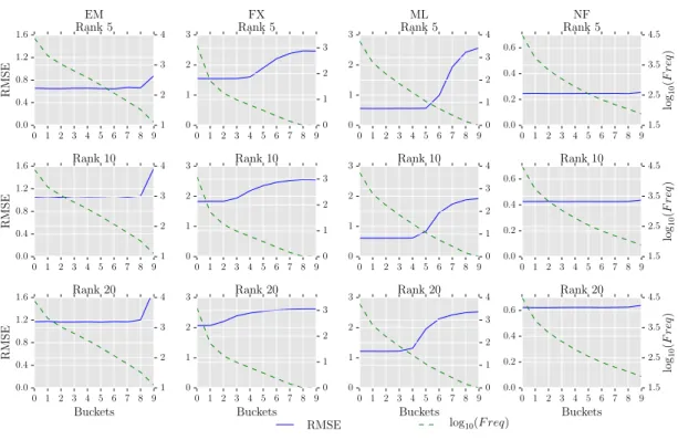
Since the matrix completion-based methods fail to recover the missing entries accurately in the SYN-REAL matrices, we investigated if the number of ratings an item has, i.e., item frequency, has any influence on the accuracy of the matrix completion-based methods for the item. We ordered all the items in decreasing order by their frequency in the rating matrix. We divided these ordered items into ten buckets and for a user computed the RMSE for items in each bucket based on the error between the predicted rating by the estimated low-rank model and the ground-truth rating. We repeated this for all the users and computed the average of the RMSE of the items in each bucket over all the users. Figure 4.1 shows the RMSEs across the buckets along with the average frequency of the items in the buckets. As can be seen in the figure, the predicted ratings for the frequent items tend to have lower RMSE in contrast to infrequent items for most
0 1 2 3 4 5 6 7 8 9 0.0 0.4 0.8 1.2 1.6 RMSE EM Rank 5 1 2 3 4 0 1 2 3 4 5 6 7 8 9 0 1 2 3 FX Rank 5 0 1 2 3 0 1 2 3 4 5 6 7 8 9 0 1 2 3 ML Rank 5 0 1 2 3 4 0 1 2 3 4 5 6 7 8 9 0.0 0.2 0.4 0.6 NF Rank 5 1.5 2.5 3.5 4.5 log 10 ( F req ) 0 1 2 3 4 5 6 7 8 9 0.0 0.4 0.8 1.2 1.6 RMSE Rank 10 1 2 3 4 0 1 2 3 4 5 6 7 8 9 0 1 2 3 Rank 10 0 1 2 3 0 1 2 3 4 5 6 7 8 9 0 1 2 3 Rank 10 0 1 2 3 4 0 1 2 3 4 5 6 7 8 9 0.0 0.2 0.4 0.6 Rank 10 1.5 2.5 3.5 4.5 log 10 ( F req ) 0 1 2 3 4 5 6 7 8 9 Buckets 0.0 0.4 0.8 1.2 1.6 RMSE Rank 20 1 2 3 4 0 1 2 3 4 5 6 7 8 9 Buckets 0 1 2 3 Rank 20 0 1 2 3 0 1 2 3 4 5 6 7 8 9 Buckets 0 1 2 3 Rank 20 0 1 2 3 4 0 1 2 3 4 5 6 7 8 9 Buckets 0.0 0.2 0.4 0.6 Rank 20 RMSE 1.5 2.5 3.5 4.5 log 10 ( F req ) log10(F req)
Figure 4.1: RMSE of the predicted ratings as the frequency of the items decreases.
of the datasets. However, in NF dataset because of the higher number of average ratings for both the users and the items the RMSE tends to remain the same over all the items. Figure 4.2 shows the scatter map of items in FX and EM dataset having different frequency against the number of instances where the absolute difference between the original and the predicted rating, i.e., Mean Absolute Error (MAE), is ≤ 0.5. As can be seen in the figure, the number of accurate predictions is significantly lower for items having fewer ratings (≤20) compared to that of the items having a greater number of ratings (≥30). The higher RMSE of the infrequent items is because they do not have sufficient ratings to estimate their latent factors accurately. Hence for the real datasets, items appearing at the top in ordering by frequency and having high predicted scores will form a reliable set of recommendations to a user.
10 20 30 40 Frequency 20000 25000 30000 35000 40000 45000 50000 No. of accurate predictions FX 0.0 0.4 0.8 1.2 1.6 2.0 2.4 2.8 3.2 log10(Coun t) 10 20 30 40 Frequency 15000 20000 25000 30000 35000 40000 No. of accurate predictions EM 0.00 0.08 0.16 0.24 0.32 0.40 0.48 0.56 0.64 0.72 log10(Coun t)
Figure 4.2: Scatter map of items having different frequency against their number of accurate predictions (Mean absolute error (MAE)≤0.5) for low-rank models with rank 20 for FX and EM datasets.
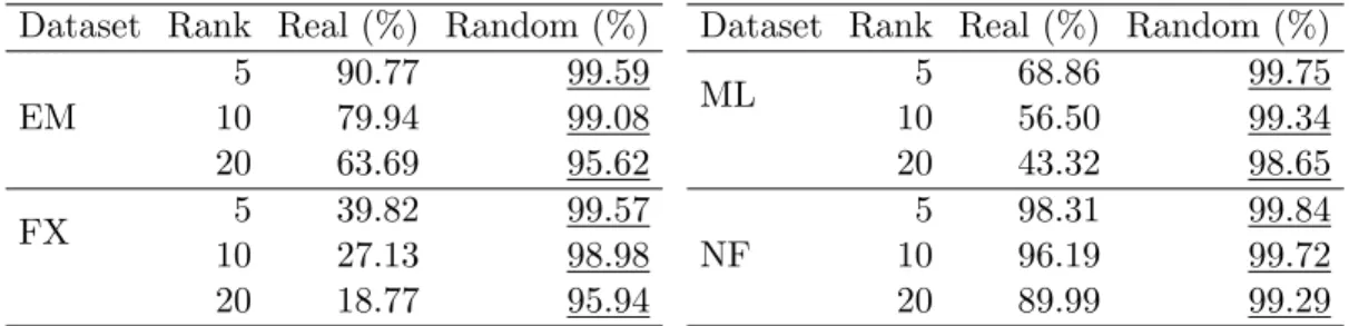
Table 4.3: Overlap between the original top 5% of the items and the predicted top 5% of the items by the estimated low-rank models for real and random sparsity structure.
Dataset Rank Real (%) Random (%)
EM 5 90.77 99.59 10 79.94 99.08 20 63.69 95.62 FX 5 39.82 99.57 10 27.13 98.98 20 18.77 95.94
Dataset Rank Real (%) Random (%)
ML 5 68.86 99.75 10 56.50 99.34 20 43.32 98.65 NF 5 98.31 99.84 10 96.19 99.72 20 89.99 99.29
4.2.3 Ranking performance of the estimated low-rank models
We define ranking performance of the estimated low-rank models as their ability to predict high the true high rated items for a user. In order to evaluate how the errors in predictions by matrix completion-based methods impact the ranking performance of the estimated low-rank model, we analyzed the top n% of the items predicted by the estimated low-rank model for a user and investigated whether true high rated items are predicted low or true low rated items are predicted high. In the following analysis, we will refer to the top n% of the items predicted by the estimated low-rank models as
Eun% and the topn% of the items ordered by the ground-truth ratings as Gnu%. Table 4.3 shows the fraction of items that are common between G5%
u and Eu5%. As
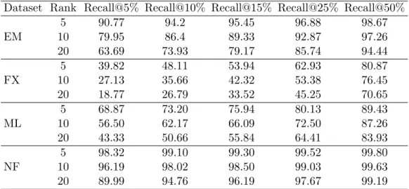
Table 4.4: Recall@n%∗ of the top 5% of the ground-truth items in rankings by the estimated low-rank models for datasets with real sparsity structure.
Dataset Rank Recall@5% Recall@10% Recall@15% Recall@25% Recall@50%
EM 5 90.77 94.2 95.45 96.88 98.67 10 79.95 86.4 89.33 92.87 97.26 20 63.69 73.93 79.17 85.74 94.44 FX 5 39.82 48.11 53.94 62.93 80.87 10 27.13 35.66 42.32 53.38 76.45 20 18.77 26.79 33.52 45.25 70.65 ML 5 68.87 73.20 75.94 80.13 89.43 10 56.50 62.17 66.09 72.50 87.26 20 43.33 50.66 55.84 64.41 83.93 NF 5 98.32 99.10 99.30 99.52 99.80 10 96.19 98.02 98.50 99.03 99.63 20 89.99 94.76 96.19 97.67 99.19
∗ The percentage of items inG5%
u that are present in Eun%.
miss a significant number of the items in G5%
u . On the contrary, the low-rank models
estimated on the matrices with random sparsity miss a comparatively smaller number of the items in G5%
u .
Further, we explored how the low-rank model mis-predicts the original top 5% items for a user, i.e., G5%u , in real datasets. We computed the position of these items in the ranking of all items by their predicted ratings and based on these positions computed the Recall@n%, i.e., the percentage of items inG5%u that are present inEun%. In Table 4.4, we present the Recall@n% of these items in the ranking of all the items by their predicted ratings. For example, as can be seen in the table for ML dataset with rank 5, the 68.87% of the items in G5%
u are present in Eu5%, 73.20% of these appear in Eu10%, and
89.43% of these are in Eu50%. Similar trend occurs for the remaining datasets, i.e., the items in G5%u that are not present inEu5% are spread across the entire ranking and this spread increases with the rank of the matrices. Also, the Recall@nis higher for denser datasets, i.e., for EM and NF, when compared to the other datasets. The lower value of Recall@5 indicates that a considerable large number of the highest rated items are not ranked high by the estimated low-rank models.
Since in many cases, E5%
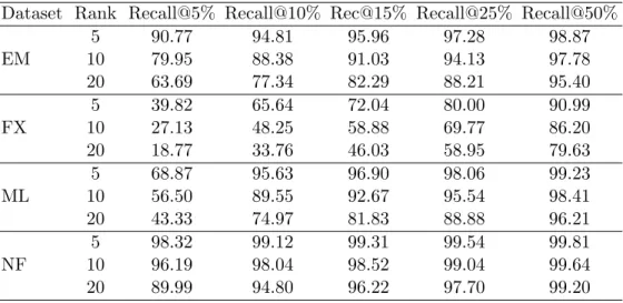
Table 4.5: Recall@n%∗ of the top 5% items predicted by low-rank models in non-increasing ordering of all items by the ground-truth ratings for datasets with real sparsity structure.
Dataset Rank Recall@5% Recall@10% Rec@15% Recall@25% Recall@50%
EM 5 90.77 94.81 95.96 97.28 98.87 10 79.95 88.38 91.03 94.13 97.78 20 63.69 77.34 82.29 88.21 95.40 FX 5 39.82 65.64 72.04 80.00 90.99 10 27.13 48.25 58.88 69.77 86.20 20 18.77 33.76 46.03 58.95 79.63 ML 5 68.87 95.63 96.90 98.06 99.23 10 56.50 89.55 92.67 95.54 98.41 20 43.33 74.97 81.83 88.88 96.21 NF 5 98.32 99.12 99.31 99.54 99.81 10 96.19 98.04 98.52 99.04 99.64 20 89.99 94.80 96.22 97.70 99.20
∗The percentage of the items inE5%
u that are present in theGnu%.
their truth ratings, we investigated where these items are located in the ground-truth rankings by computing the position of the items in E5%
u in the ranking of all
items by their ground truth ratings. We computed the Recall@n% of these items, i.e., the percentage of the items in Eu5% that are present in the Gnu%. Table 4.5 shows the Recall@n% of the items inE5%
u in the ranking of all items by the ground-truth ratings
in decreasing order. For example, as can be seen in the table for ML dataset with rank 5, the 68.87% of items inE5%
u are present inG5%u , 95.63% of these appear inG10%u , and
almost all, i.e., 99.23% of these are inG50%u . The remaining datasets in the table follows a similar trend, i.e., the items in Eu5% are present close to the top in the ground-truth ranking. This indicates that the items that are predicted high by the estimated low-rank models are also in general true high rated items.
Effect of item frequency
We investigated how the ranking performance of the estimated low-rank models varies with the frequency of the items in SYN-REAL matrices.
To this end, for each user we computed the Recall@n% of the items in G5%u , i.e., the percentage of the items inG5%
5 10 15 0 20 40 60 80 100 Recall@ n % EM Rank 5 1080 1120 1160 1200 25 50 75 0 20 40 60 80 100 FX Rank 5 0 50 100 150 200 250 25 50 0 20 40 60 80 100 ML Rank 5 0 200 400 600 800 5 10 0 20 40 60 80 100 NF Rank 5 3750 3850 3950 4050 4150 F req@ n % 5 10 15 20 25 30 0 20 40 60 80 100 Recall@ n % Rank 10 1080 1120 1160 1200 1240 25 50 75 0 20 40 60 80 100 Rank 10 0 100 200 300 25 50 0 20 40 60 80 100 Rank 10 0 400 800 1200 5 10 0 20 40 60 80 100 Rank 10 3950 4000 4050 4100 4150 4200 F req@ n % 10 20 30 40 50 n 0 20 40 60 80 100 Recall@ n % Rank 20 950 1050 1150 1250 25 50 75 n 0 20 40 60 80 100 Rank 20 0 100 200 300 400 25 50 75 n 0 20 40 60 80 100 Rank 20 0 400 800 1200 5 10 15 n 0 20 40 60 80 100 Rank 20 Recall@n 3900 4100 4300 4500 F req@ n % Freq@n%
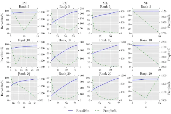
Figure 4.3: Recall@n% and Freq@n% of the top 5% of the ground-truth items in ordering by the predictions from the estimated low-rank models.
[5, 10, 15, ..., 100]. Also, we computed the average frequency of the items in G5%u that are present in Eun% but are absent in Eu(n−5)%. We will refer to the average frequency
of these items as Freq@n%. As can be seen in Figure 4.3, for the datasets with fewer ratings per item, i.e., the ML and the FX datasets, the items having low frequency tend to appear at the end of the ranking. This trend is also seen to some extent in the denser datasets, i.e., the EM and the NF datasets. We hypothesize that it is because the low-rank model, i.e., the user and the item latent factors, is initialized with values close to zero and since items with fewer ratings do not often occur in the updates during the model estimation they are predicted low by the estimated low-rank model. Therefore, the ranking performance of the estimated low-rank models on SYN-REAL matrices is not affected by false positives as both frequent and infrequent items that are rated low will be predicted low while frequent items that are rated high will be predicted high. To test this hypothesis, we initialized the low-rank models with higher values in the range
5 10 15 0 20 40 60 80 100 Recall@ n % EM Rank 5 1100 1140 1180 1220 25 50 75 0 20 40 60 80 100 FX Rank 5 0 100 200 300 10 20 30 40 50 0 20 40 60 80 100 ML Rank 5 200 400 600 800 5 10 0 20 40 60 80 100 NF Rank 5 3900 4000 4100 4200 F req@ n % 10 20 30 40 0 20 40 60 80 100 Recall@ n % Rank 10 700 900 1100 1300 25 50 75 0 20 40 60 80 100 Rank 10 0 100 200 300 400 25 50 0 20 40 60 80 100 Rank 10 0 200 400 600 800 5 10 0 20 40 60 80 100 Rank 10 4000 4040 4080 4120 4160 F req@ n % 25 50 75 n 0 20 40 60 80 100 Recall@ n % Rank 20 1150 1200 1250 1300 1350 1400 25 50 75 n 0 20 40 60 80 100 Rank 20 0 100 200 300 400 500 25 50 75 n 0 20 40 60 80 100 Rank 20 0 200 400 600 800 5 10 15 20 25 n 0 20 40 60 80 100 Rank 20 Recall@n 3900 4100 4300 4500 F req@ n % Freq@n%
Figure 4.4: Recall@n% and Freq@n% of the top 5% of the ground-truth items in ordering by the predictions from the estimated low-rank models initialized with values in the range [0, 5].
[0,5] and analyzed the learned models. Figure 4.4 shows the Recall@n% of the items in G5%
u along with their average frequency, i.e., Freq@n%, for the estimated low-rank
models initialized with higher values. As can be seen in the figure, unlike the estimated low-rank models initialized with values close to zero, the items having low frequency does not necessarily appear in the later buckets. Additionally, the Recall@n is significantly lower for smaller values ofnwhen compared with that of the estimated low-rank models initialized with values close to 0. This suggests that the model initialization affects both the accuracy and the ranking performance of the matrix completion-based methods.
Previously in Section 4.2.2, we showed that the accuracy of the estimated low-rank models is better for items having high frequency. Considering the analysis of ranking performance, we can reason that the frequent items that are rated high will be predicted high by the estimated low-rank model. Hence, the ranking performance of the estimated
low-rank model is better for these items than the items that are rated high but are infrequent.
4.3
Conclusion
In this work, we have investigated the performance of the matrix completion-based low-rank models for estimating the missing ratings in user-item rating matrices having sparsity structure identical to real datasets. We showed in Section 4.2.2 that the matrix completion-based methods because of the presence of skewed distribution of entries in rating matrices in real datasets fail to predict the missing entries accurately in the matrices. Also, we learned that the items with high frequency are predicted more accurately than the others. These findings imply that for a user, the unrated items which have more ratings in the matrix and are predicted high for the user, will form a better set of recommendations than the items with fewer ratings in the rating matrix.
Further, we saw in Section 4.2.3 that the errors in predictions due to the skewed distribution of ratings in the user-item rating matrix affect the ranking performance of the matrix-completion based methods. In particular, under the assumption that the rating that a user will provide to an item determines his ranking preference, our results indicate that the items predicted at the top by matrix completion-based methods miss a large number of true high rated items. In some datasets, the true high rated items are missing even in the top 50% of the predicted items for the user. However, the items that are predicted at the top for a user but are absent from the true high rated items are present close to the true high rated items by the user. Therefore, the ranking based on the predicted ratings is not severely affected by false positives as it does not contain items that are significantly low rated. Additionally, we observed that the infrequent items, irrespective of whether they are true high rated or true low rated, are predicted low by the matrix completion-based methods thereby appearing later in the ranking of the items for recommendations.
Chapter 5
TruncatedMF: Truncated matrix
factorization
This chapter focuses on improving the matrix completion-based recommendation meth-ods for users and items present in the tail, i.e., those having few ratings in the user-item rating matrix. We show that the performance of matrix completion in real datasets vary with the number of ratings that a user or an item has, and its accuracy is low for the users or the items with few rating. Furthermore, we use these insights to develop Trun-catedMF, a matrix completion-based approach, that outperforms the state-of-the-art MF method for the users and the items in the tail.
5.1
Introduction
The matrix completion-based methods, e.g., matrix factorization (MF) [10, 11, 14], are the state-of-the-art collaborative filtering methods that use users’ historical preferences over items to generate recommendations. The ratings provided by users over the items can be viewed as a matrix whose rows represent the users, columns denote the items, and entries are the ratings provided by the users over the items. There exists a small number of attributes that describe the items, and a user’s rating depends on how the user values those attributes. This makes the user-item rating matrix low-rank, and the number of attributes determines the rank of the matrix. The attributes of the items and the weights provided by a user over these attributes are often referred as the items’
Table 5.1: Datasets used in experiments
Dataset users items ratings µua σub µic σid density
(%)† EachMovie (EM) 61,265 1,623 2,811,983 45.89 59.48 1732.58 3882.55 2.8 Flixster (FX) 147,612 48,794 8,196,077 55.52 225.81 167.97 934.47 0.1 Movielens 10M (ML10) 69.878 10,677 10,000,054 143.10 216.71 936.59 2487.21 0.01 Movielens 20M (ML20) 229,060 26,779 21,063,128 91.95 190.53 786.55 3269.45 0.3 Netflix (NF) 480,189 17,772 100,480,507 209.252 302.33 4550.75 16908.40 1.1
aThe number of average ratings per user in the dataset. bThe standard deviation of ratings per user in the dataset. c The number of average ratings per item in the dataset. dThe standard deviation of ratings per item in the dataset. † The percentage of observed ratings in the dataset.
latent factors and the users’ latent factors, respectively. MF estimates the user-item rating matrix as the product of the user latent factors and the item latent factors.
In practice, there are few attributes that are responsible for a large portion of the rating provided by a user on an item and the remaining rating can be explained by other attributes. However, certain users have provided ratings to few items, and some items have received few ratings from the users thereby these users or items may not have sufficient ratings to estimate weights for all the attributes accurately. The inaccuracy in the estimation of weights for these users and items can affect the predicted ratings and hence affect the generated recommendations. Therefore, the recommendations for these users and items with few ratings may improve by focusing on few attributes that are responsible for a significant portion of the rating and can be estimated accurately by matrix completion-based methods.
This chapter investigates how does the performance of the matrix completion-based methods changes with the number of ratings that a user or an item has, and shows that the users or the items with few ratings tend to have low accuracy. Additionally, we show that the error in predictions for such users or items increases further with the increase in rank of the low-rank matrix completion-based methods. Furthermore, we use these findings to develop TruncatedMF which considers the number of ratings received by an item or provided by a user to estimate the rating of the user on the item. The exhaustive experiments on the real datasets demonstrate the effectiveness of TruncatedMF over the state-of-the-art MF method for the users and the items with few ratings.
5.2
Effect of frequency on accuracy in real datasets
We investigated how does the performance of matrix completion method vary for items with the different number of ratings in user-item rating matrix and in order to do the analysis we evaluated matrix completion on a random held-out subset of the real datasets shown in Table 5.1. We followed the standard procedure of dividing the available ratings in a dataset at random into training, validation and test splits, i.e., 60% of the ratings were used for learning the low-rank models and rest were used equally for validation and test splits. To learn the model we tried rank in the range [1, 5, 10, 15, 25, 30, 40, 50] and regularization parameters in the range [0.001, 0.01, 0.1, 1]. We performed this procedure three times and selected the model giving the lowest average RMSE on the validation splits. Table 5.2 shows the test RMSE achieved by the selected models for different datasets. In addition to computing RMSE over all the ratings in the test split, we also computed RMSE over the infrequent items in the test split, i.e., the items that have few ratings in the training split. In order to identify infrequent items, we ordered the items in increasing order by the number of ratings in training splits. Next, we divided these ordered items into quartiles and designated the items in the first and the last quartile as the infrequent and the frequent items respectively.
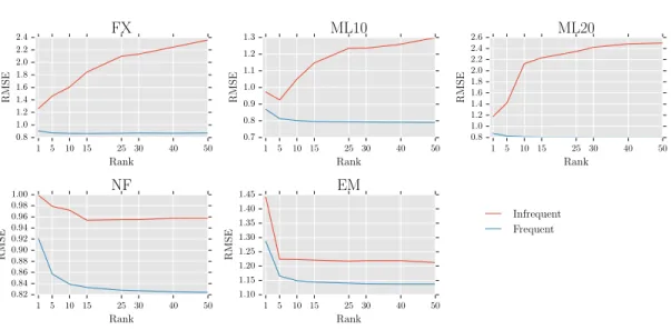
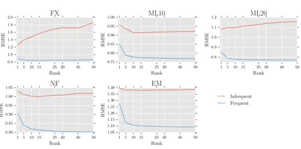
Figures 5.1 and 5.2 show the RMSE for the items and the users in the test, respec-tively. As can be seen in the figures, for all the datasets the RMSE of the frequent items (or users) is lower than that of the infrequent items (or users) . These results suggest that the matrix completion method fails to estimate the preferences for the infrequent items (or users) accurately in the real datasets. Also as can be seen in Figure 5.1, for FX, ML10 and ML20 datasets, the RMSE of the infrequent items increases with the increase in the rank while that of frequent items decreases with the increase in the rank. Since NF and EM has a high number of average ratings for the items, the RMSE also tends to decrease for the infrequent items with the increase in the rank. Similarly, as can be seen in Figure 5.2, in FX and ML20 datasets the RMSE of the infrequent users increases with the increase in the rank. The increase in RMSE with the increase in ranks suggests that infrequent items or infrequent users may not have sufficient ratings to estimate all the ranks accurately thereby leading to the error in predictions for such users or items.
Table 5.2: Test RMSE for real datasets. Rank EM FX ML10 ML20 NF 1 1.282 0.903 0.870 0.875 0.926 5 1.158 0.871 0.815 0.824 0.863 10 1.142 0.866 0.804 0.813 0.845 15 1.138 0.864 0.800 0.810 0.839 25 1.134 0.864 0.798 0.809 0.834 30 1.132 0.864 0.797 0.809 0.832 40 1.132 0.864 0.796 0.809 0.831 50 1.131 0.864 0.796 0.809 0.830
5.3
Truncated matrix factorization
In Section 5.2, we showed that the infrequent items and the infrequent users tend to have a high error under matrix completion-based approach. Furthermore, this error increases with the increase in rank of the estimated low-rank models, i.e, increases with the dimension of estimated users’ and items’ latent factors. We propose to use these observations to devise a approach, which we will refer to as Truncated Matrix Factorization (TMF), to improve the accuracy of the low-rank models for both the users and the items having few ratings. Since for the items and the users with few ratings we may not be able to estimate all the ranks of a low-rank model accurately, we propose to consider only a subset of the ranks for these users or items.
In our approach, the estimated rating for useru on itemiis given by
ˆ
ru,i =pu(qihu,i)T, (5.1)
where pu denotes the latent factor of user u, qi represents the latent factor of item i,
hu,i is a vector containing 1s in the beginning followed by 0s, and represents the
elementwise Hadamard product between the vectors. The vector hu,i is used to select
the ranks that are active for the (u, i) tuple. The 1s inhu,i denote the active ranks for
1 5 10 15 25 30 40 50 Rank 0.8 1.0 1.2 1.4 1.6 1.8 2.0 2.2 2.4 RMSE FX 1 5 10 15 25 30 40 50 Rank 0.7 0.8 0.9 1.0 1.1 1.2 1.3 RMSE ML10 1 5 10 15 25 30 40 50 Rank 0.8 1.0 1.2 1.4 1.6 1.8 2.0 2.2 2.4 2.6 RMSE ML20 1 5 10 15 25 30 40 50 Rank 0.82 0.84 0.86 0.88 0.90 0.92 0.94 0.96 0.98 1.00 RMSE NF 1 5 10 15 25 30 40 50 Rank 1.10 1.15 1.20 1.25 1.30 1.35 1.40 1.45 RMSE EM Infrequent Frequent
Figure 5.1: Test RMSE of the frequent and infrequent items in real datasets.
5.3.1 Frequency adaptive truncation
A way to select the active ranks, i.e.,hu,ifor a user-item rating is based on the frequency
of the user and the item in the rating matrix. In this approach, for a given rating by a user on an item, first, we determine the number of ranks to be updated based on either the user or the item depending on the one having a lower number of ratings. In order to select the ranks, we normalize the frequency of the user and the item, and use a non-linear activation function, e.g., sigmoid function, to map this frequency of the user or the item in [0, 1]. Finally, we use the product of the output of the activation function and rank of the low-rank model as the number of active ranks selected for the (u, i) tuple. The number of active ranks to be selected is given by
ku,i = r 1+e−k(fu−z), iffu ≤fi r 1+e−k(fi−z), otherwise, (5.2)
where r is the rank of the low-rank model, i.e., dimension of the user and the item latent factors, fu is the frequency of user u, fi is the frequency of item i, k controls
1 5 10 15 25 30 40 50 Rank 0.8 1.0 1.2 1.4 1.6 1.8 2.0 RMSE FX 1 5 10 15 25 30 40 50 Rank 0.75 0.80 0.85 0.90 0.95 1.00 RMSE ML10 1 5 10 15 25 30 40 50 Rank 0.8 0.9 1.0 1.1 1.2 RMSE ML20 1 5 10 15 25 30 40 50 Rank 0.80 0.85 0.90 0.95 1.00 1.05 RMSE NF 1 5 10 15 25 30 40 50 Rank 1.05 1.10 1.15 1.20 1.25 1.30 1.35 1.40 RMSE EM Infrequent Frequent
Figure 5.2: Test RMSE of the frequent and infrequent users in real datasets.
additional motivation for using a non-linear activation function, e.g., sigmoid function, is that the shape of the plot in Figure 4.2 is non-linear. Hence, using such a function assists in identifying the users or the items for whom we may estimate only a few ranks accurately. The active ranks to be selected are given by
hu,i[j]= 1, ifj≤ku,i 0, otherwise. (5.3)
We will refer to this method as Truncated matrix factorization (TMF).
5.3.2 Frequency adaptive probabilistic truncation
An alternative way to select the active ranks is to assume that the number of active ranks follows a Poisson distribution with parameter ku,i. This method is similar to
Dropout [65] technique in neural networks, where parameters are selected probabilisti-cally for updates during learning of the model. Similar to regularization it provides a way of preventing overfitting in learning of the model. The active ranks to be selected
Algorithm 1 Learn TMF
1: procedure LearnTMF
2: r←rank of low-rank models 3: η←learning rate
4: λ←regularization parameter 5: k←steepness constant 6: z←mid-point
7: R ←all users’ ratings on items 8: f ←users’ and items’ frequency 9: iter←0
10: InitP,Qwith random values∈ [-0.01, 0.01]
11: whileiter<maxIter or error on validation set decreases do
12: for each ru,i ∈ Rdo
13: if fu≤fi then 14: ku,i ← r 1+e−k(fu−z) 15: else 16: ku,i ← r 1+e−k(fi−z) 17: end if 18: hu,i ←1 19: for each doj ∈[1, r] 20: if j > ku,i then 21: hui[j]←0 22: end if 23: end for 24: rˆu,i=pu(qihu,i)T
25: eu,i←rˆu,i−ru,i
26: for each j∈[1, ku,i]do
27: pu[j]←pu[j]−η(2eu,iqi[j] + 2λpu[j]) 28: qi[j]←qi[j]−η(2eu,ipu[j] + 2λqi[j]) 29: end for 30: end for 31: end while 32: returnP, Q 33: end procedure
Algorithm 2 Learn TMF + Dropout
1: procedure LearnTMFDropout
2: r←rank of low-rank models 3: η←learning rate
4: λ←regularization parameter 5: k←steepness constant 6: z←mid-point
7: R ←all users’ ratings on items 8: f ←users’ and items’ frequency 9: iter←0
10: InitP,Qwith random values∈ [-0.01, 0.01]
11: whileiter<maxIter or error on validation set decreases do
12: for each ru,i ∈ Rdo
13: if fu≤fi then 14: ku,i ← r 1+e−k(fu−z) 15: else 16: ku,i ← 1+e−k(rfi−z) 17: end if 18:
19: θu,i∼P oisson(ku,i) 20: hu,i ←1 21: for each doj ∈[1, r] 22: if j > θu,i then 23: hui[j]←0 24: end if 25: end for 26: rˆu,i=pu(qihu,i)T
27: eu,i←rˆu,i−ru,i
28: for each j∈[1, θu,i]do
29: pu[j]←pu[j]−η(2eu,iqi[j] + 2λpu[j]) 30: qi[j]←qi[j]−η(2eu,ipu[j] + 2λqi[j]) 31: end for 32: end for 33: end while 34: returnP, Q 35: end procedure
are given by hu,i[j]= 1, ifj≤θu,i 0, otherwise,
where θu,i∼P oisson(ku,i) and ku,i is given by Equation 5.2. We will call this method
as Truncated matrix factorization with Dropout (TMF + Dropout).
5.3.3 Model learning
The parameters of the model, i.e., the user and the item latent factors, can be estimated by minimizing Equation 3.2 as described in Section 3. Algorithms 1 and 2 provides the detailed procedure for TMF and TMF + Dropout, respectively.
5.3.4 Rating prediction
After learning the model the predicted rating for a user u on a item ifor TMF model is given by
ˆ
ru,i =pu(qihu,i)T, (5.4)
where the active ranks, i.e., hu,i, is given by Equation 5.3. The predicted rating for
the user and the item under TMF + Dropout model is given by the least number of ranks for whom the cumulative distribution function (CDF) for Poisson distribution with parameter kui obtains approximately the value of 1. The active ranks, i.e., hu,i,
used for prediction under TMF + Dropout are given by
hu,i[j]= 1, ifj≤s 0, otherwise, (5.5)
where s is the least number of ranks for whom the CDF, i.e, P(x <= s) ≈ 1, x ∼ P oisson(ku,i) andku,i is given by Equation 5.2.
![Figure 4.4: Recall@n% and Freq@n% of the top 5% of the ground-truth items in ordering by the predictions from the estimated low-rank models initialized with values in the range [0, 5].](https://thumb-us.123doks.com/thumbv2/123dok_us/1995708.2796438/37.918.215.789.204.583/figure-recall-ground-ordering-predictions-estimated-models-initialized.webp)