Two-Stage Metric Learning
Jun Wang [email protected]
Department of Computer Science, University of Geneva, Switzerland
Ke Sun [email protected]
Department of Computer Science, University of Geneva, Switzerland
Fei Sha [email protected]
Department of Computer Science, University of Southern California, Los Angeles, CA, USA
Stephane Marchand-Maillet [email protected]
Department of Computer Science, University of Geneva, Switzerland
Alexandros Kalousis [email protected]
Department of Business Informatics,University of Applied Sciences,Western Switzerland, Department of Computer Science, University of Geneva, Switzerland
Abstract
In this paper, we present a novel two-stage metric learning algorithm. We first map each learning instance to a probability distribution by comput-ing its similarities to a set of fixed anchor points. Then, we define the distance in the input data space as the Fisher information distance on the associated statistical manifold. This induces in the input data space a new family of distance metric with unique properties. Unlike kernelized metric learning, we do not require the similarity measure to be positive semi-definite. Moreover, it can also be interpreted as a local metric learn-ing algorithm with well defined distance approx-imation. We evaluate its performance on a num-ber of datasets. It outperforms significantly other metric learning methods and SVM.
1. Introduction
Distance measures play a crucial role in many machine learning tasks and algorithms. Standard distance metrics, e.g. Euclidean, cannot address in a satisfactory manner the multitude of learning problems, a fact that led to the devel-opment of metric learning methods which learn
problem-specific distance measure directly from the data (
Wein-berger & Saul,2009;Wang et al.,2012;Jain et al.,2010).
Proceedings of the 31st International Conference on Machine Learning, Beijing, China, 2014. JMLR: W&CP volume 32. Copy-right 2014 by the author(s).
Over the last years various metric learning algorithms have been shown to perform well in different learning problems, however, each comes with its own set of limitations. Learning the distance metric with one global linear trans-formation is called single metric learning (Weinberger & Saul,2009; Davis et al.,2007). In this approach the dis-tance computation is equivalent to applying on the learn-ing instances a learned linear transformation followed by a standard distance metric computation in the projected space. Since the discriminatory power of the input fea-tures might vary locally, this approach is often not flexible enough to fit well the distance in different regions. Local metric learning addresses this limitation by
learn-ing in each neighborhood one local metric (Noh et al.,
2009; Wang et al., 2012). When the local metrics vary smoothly in the feature space, learning local metrics is equivalent to learning the Riemannian metric on the data
manifold (Hauberg et al.,2012). The main challenge here
is that the geodesic distance endowed by the Riemannian metric is often computationally very expensive. In practice, it is approximated by assuming that the geodesic curves are formed by straight lines and the local metric does not
change along these lines (Noh et al., 2009; Wang et al.,
2012). Unfortunately, the approximation does not satisfy
the symmetric property and therefore the result is a non-metric distance.
Kernelized Metric Learning (KML) achieves flexibility in
a different way (Jain et al., 2010; Wang et al., 2011).
In KML learning instances are first mapped into the Reproducing-Kernel Hilbert Space (RKHS) by a kernel
Learning (ICML), Beijing, China, 21-26 June 2014, p.370-378 which should be
cited to refer to this work
function and then a global Mahalanobis metric is learned in the RKHS space. By defining the distance in the input fea-ture space as the Mahalanobis distance in the RKHS space, KML is equivalent to learning a flexible non-linear distance in the input space. However, its main limitation is that the kernel matrix induced by the kernel function must be Posi-tive Semi-Definite (PSD). Although Non-PSD kernel could
be transformed into PSD kernel (Chen & Ye,2008;Ying
et al.,2009), the new PSD kernel nevertheless cannot keep all original similarity information.
In this paper, we propose a novel two-stage metric learn-ing algorithm, Similarity-Based Fisher Information Metric Learning (SBFIML). It first maps instances from the data manifold into finite discrete distributions by computing their similarities to a number of predefined anchor points in the data space. Then, the Fisher information distance on the statistical manifold is used as the distance in the input feature space. This induces a new family of Riemannian distance metric in the input data space with two important properties. First, the new Riemannian metric is robust to density variation in the original data space. Without such robustness, an objective function can be easily biased to-wards data regions the density of which is low and thus dominates learning of the objective function. Second, the new Riemannian metric has largest distance discrimination on the manifold of anchor points and no distance in the di-rections being orthogonal to the manifold. So, the effect of locally irrelevant dimensions of anchor points is removed. To the best of our knowledge, this is the first metric learn-ing algorithm that has these two important properties. SBFIML is flexible and general; it can be applied to dif-ferent types of data spaces with various non-negative sim-ilarity functions. Comparing to KML, SBFIML does not require the similarity measure to form a PSD matrix. More-over, SBFIML can be interpreted as a local metric learning algorithm. Compared to the previous local metric
learn-ing algorithms which produce a non-metric distance (Noh
et al.,2009; Wang et al., 2012), the distance approxima-tion in SBFIML is a well defined distance funcapproxima-tion with a closed form expression. We evaluate SBFIML on a num-ber of datasets. The experimental results show that it out-performs in a statistically significant manner both metric learning methods and SVM.
2. Preliminaries
We are given a number of learning instances{x1, . . . ,xn},
where each instance xT
i ∈ X is a d-dimensional vector,
and a vector of associated class labelsy= (y1, . . . , yn)T,
yi ∈ {1, . . . , c}. We assume that the input feature spaceX
is a smooth manifold. Different learning problems can have very different types of data manifolds with possibly differ-ent dimensionality. The most commonly used manifold in
metric learning is the Euclidean spaceRd (Weinberger &
Saul,2009). The probability simplex spacePd−1has also
been explored (Lebanon,2006;Cuturi & Avis,2011; Ke-dem et al.,2012).
We propose a general two-stage metric learning algorithm
which can learn a flexible distance in different types ofX
data manifolds, e.g. Euclidean, probability simplex,
hyper-sphere, etc. Concretely, we first map instances fromXonto
the statistical manifoldSthrough a similarity-based differ-ential map, which computes their non-negative similarities to a number of predefined anchor points. Then we define
the Fisher information distance as the distance onX. We
have chosen to do so, since this induces a new family of Riemannian distance metric which enjoys interesting prop-erties: 1) The new Riemannian metric is robust to density variations in the original data space, which can be produced for example by different intrinsic variabilities of the learn-ing instances in the different categories. Distance learnlearn-ing over this new metric is hence robust to density variation. 2) The new Riemannian distance metric has largest dis-tance discrimination on the manifold of the anchor points and has no distance in the directions being orthogonal to that manifold. So, the new distance metric can remove the effect of locally irrelevant dimensions of the anchor point
manifold, see Figure1 for more detials. In the remainder
of this section, we will briefly introduce the necessary ter-minology and concepts. More details can be found in the monographs (Lee,2002;Amari & Nagaoka,2007).
Statistical Manifold. We denote byMnan-dimensional
smooth manifold. For each point ponMn, there exists
at least one smooth coordinate chart(U, ϕ)which defines
a coordinate system to points on U, where U is an open
subset ofMncontainingpandϕ: U −→ Θis a smooth
coordinate mapϕ(p) = θ ∈Θ⊂Rn.θis the coordinate
ofpdefined byϕ.
A statistical manifold is a smooth manifold whose points are probability distributions. Given an-dimensional statis-tical manifoldSn, we denote byp(ξ|θ)a probability
dis-tribution inSn, whereθ = (θ
1, . . . , θn)∈Θ⊂Rn is the
coordinate ofp(ξ|θ)under some coordinate mapϕandξis the random variable of thep(ξ|θ)distribution taking values from some setΞ. Note that, all the probability distributions inSnshare the same setΞ.
In this paper, we are particularly interested in the n
-dimensional statistical manifoldPn, whose points are finite
discrete distributions, denoted by
Pn={p(ξ|θ= (θ1, . . . , θn)) : n
X
i=1
θi<1,∀i, θi>0} (1)
whereξ is the discrete random variable taking values in
the set Ξ = {1, . . . , n+ 1} andθ ∈ Θ ⊂ Rn is called
probability mass ofp(ξ|θ)isp(ξ =i) =θiifi6=n+ 1,
otherwisep(ξ=n+ 1) = 1−Pn
k=1θk.
Fisher Information Metric. The Fisher information met-ric is a Riemannian metmet-ric defined on statistical mani-folds and endows a distance between probability
distribu-tions (Radhakrishna Rao,1945). The explicit form of the
Fisher information metric at p(ξ|θ) is a n×n positive
definite symmetric matrixGF IM(θ), the(i, j)element of
which is defined by: GijF IM(θ) = Z Ξ ∂logp(ξ|θ) ∂θi ∂logp(ξ|θ) ∂θj p(ξ|θ)dξ (2)
where the above integral is replaced with a sum ifΞis
dis-crete. The following lemma gives the explicit form of the
Fisher information metric onPn.
Lemma 1. On the statistical manifoldPn, the Fisher
in-formation metricGF IM(θ)atp(ξ|θ)with coordinateθis
GijF IM(θ) = 1 θi δij+ 1 1−Pn k=1θk ,∀i, j∈ {1, . . . , n} (3) whereδij= 1ifi=j, otherwiseδij = 0.
Properties of Fisher Information Metric. The Fisher information metric enjoys a number of interesting prop-erties. First, the Fisher information metric is the unique
Riemannian metric induced by allf-divergence measures,
such as the Kullback-Leibler (KL) divergence and theχ2
divergence (Amari & Cichocki, 2010). All these
diver-gences converge to the Fisher information distance as the two probability distributions are approaching each other. Another important property of the Fisher information met-ric from a metmet-ric learning perspective is that the distance it endows can be approximated by the Hellinger distance, the cosine distance and allf-divergence measures (Kass &
Vos,2011). More importantly, whenSn is the statistical
manifold of finite discrete distributions, e.g.Pn, the cosine
distance is exactly equivalent to the Fisher information dis-tance (Lebanon,2006;Lee et al.,2007).
Pullback Metric. LetMnandNmbe two smooth
mani-folds andTpMnbe the tangent space ofMn atp∈ Mn.
Given a differential mapf :Mn−→ Nmand a
Rieman-nian metric GonNm, the differential map f induces a
pullback metricG∗at each pointponMndefined by:
hv1,v2iG∗(p)=hDpf(v1), Dpf(v2)iG(f(p)) (4)
whereDpf :TpMn −→ Tf(p)Nmis the differential off
at pointp∈ Mn, which maps tangent vectorsv∈ T
pMn
to tangent vectorsDpf(v)∈ Tf(p)Nm.
Given the coordinate systems ΘandΓof U ⊂ Mn and
U0⊂ Nmrespectively, defined by some smooth coordinate
mapsϕU andϕU0 respectively, then the explicit form of
the pullback metric at pointp∈ U ⊂ Mn with coordinate
θ=ϕU(p)is:
G∗(θ) =JTG(γ)J (5)
whereγ=ϕU0(f(p))is the coordinate of thef(p)∈ U0 ⊂
NmandJis the Jacobian matrix of the functionϕ
U0 ◦f ◦
ϕ−U1: Θ−→Γat pointθ. SinceGis a Riemannian metric,
the pullback metricG∗is in general at least a PSD metric.
The following lemma gives the relation between the
geodesic distances onMnandNm.
Lemma 2. LetG∗be the pullback metric of a Riemannian metricGinduced by a differential mapf :Mn −→ Nm,
dG∗(p0, p) be the geodesic distance onMn endowed by
G∗anddG(f(p0), f(p))the geodesic distance onNm en-dowed byG, then, it holdslimp0→pdG(f(p
0),f(p))
dG∗(p0,p) = 1
The proof of Lemma2is provided in the appendix. In
ad-dition to approximatingdG∗(p0, p)directly onMnby
as-suming that the geodesic curve is formed by straight lines as previous local metric learning algorithms do (Noh et al.,
2009;Wang et al.,2012), Lemma2 allows us to also ap-proximate it withdG(f(p0), f(p))onNm. Note that, both
approximations have the same asymptotic convergence re-sult.
3. Similarity-Based Fisher Information
Metric Learning
We will now present our two-stage metric learning algo-rithm, SBFIML. In the following, we will first present how
to define the similarity-based differential mapf :X −→ P
and then how to learn the Fisher information distance.
3.1. Similarity-Based Differential Map
Given a number of anchor points{z1, . . . ,zn},zi ∈ X,
we denote bys= (s1, . . . , sn) :X −→R+nthe
differen-tiable similarity function. Eachsk:X −→R+component
is a differentiable function the output of which is a
non-negative similarity between some input instancexiand the
anchor pointzk. Based on the similarity functionswe
de-fine the similarity-based differential mapfas: f(xi) =p(ξ|( s1(xi) Pn k=1sk(xi) , . . . ,Psnn−1(xi) k=1sk(xi) ))(6) = (¯s1(xi), . . . ,¯sn−1(xi))
where f(xi) is a finite discrete distribution on manifold
Pn−1. From now on, for simplicity, we will denotef(x i)
bypi(ξ). The probability mass of thekth outcome is given
by: pi(ξ =k) = ¯s k(xi) =
sk(xi)
Pn
k=1sk(xi). In order forf to
be a valid differential map, the similarity functionsmust
satisfyP
ksk(xi)>0, ∀xi ∈ X. This family of
where a non-negative differentiable similarity function s can be defined. The finite discrete distribution representa-tion,pi(ξ), of learning instance,x
i, can be intuitively seen
as an encoding of its neighborhood structure defined by the
similarity functions. Note that, the idea of mapping
in-stances onto the statistical manifoldP has been previously
studied in manifold learning, e.g. SNE (Hinton & Roweis,
2002) and t-SNE (Van der Maaten & Hinton,2008). Akin to the appropriate choice of the kernel function in a kernel-based method, the choice of an appropriate
similar-ity functionsis also crucial for SBFIML. In principle, an
appropriate similarity functionsshould be a good match
for the geometrical structure of theX data manifold. For
example, for data lying on the probability simplex space,
i.e. X = Pd−1, the similarity functions defined either
onRd or onPd−1 can be used. However, the similarity
function onPd−1 is more appropriate, because it exploits
the geometrical structure ofPd−1, which, in contrast, is
ignored by the similarity function on Rd (Kedem et al.,
2012).
The set of anchor points {z1, . . . ,zn} can be defined in
various ways. Ideally, anchor points should be similar to
the given learning instancesxi, i.e. anchor points follow
the same distribution as that of learning instances. Empiri-cally, we can use directly training instances or cluster cen-ters, the latter established by clustering algorithms. Similar to the current practice in kernel methods we will use in SB-FIML as anchors points all the training instances.
Similarity Functions onRd.We can define the similarity
onRdin various ways. In this paper we will investigate two
types of differentiable similarity functions. The first one is based on the Gaussian function, defined as:
sk(xi) =exp(−
kxi−zkk22
σk
) (7)
wherek · k2 is theL2 norm. σk controls the size of the
neighborhood of the anchor pointzk, with large values
pro-ducing large neighborhoods. Note that the different σks
could be set to different values; if all of them are equal, this similarity function is exactly the Gaussian kernel. The second type of similarity function that we will look at is:
sk(xi) = 1− 1 πarccos( xT izk kxik2· kzkk2 ) (8)
which measures the normalized angular similarity between
xiandzk. This similarity function can be explained as we
first projecting all points fromRd to the hypersphere and
then applying the angular similarity to points on a hyper-sphere. As a result, this similarity function is useful for data which approximately lie on a hypersphere. Note that this similarity function is also a valid kernel function (Honeine & Richard,2010).
One might say we can also achieve nonlinearity by
map-ping instances into the proximity space Qusing the
fol-lowing similarity-based mapg:X −→ Q:
g(x) = (s1(x), . . . , sn(x)) (9)
We now compare our similarity-based mapf, equation6
against the similarity-based mapg, equation9, in two
as-pects, namely representation robustness and pullback met-ric analysis.
Representation Robustness. Compared to the
represen-tation induced by the similarity-based mapg, equation9,
our representation induced by the similarity-based mapf,
equation 6, is more robust to density variations in
origi-nal data space, i.e. the density of the learning instances varies significantly between different regions. This can be explained by the fact that the finite discrete distribution is essentially a representation of the neighborhood structure of a learning instance normalized by a ”scaling” factor, the sum of similarities of the learning instance to the anchor points. Hence the distance implied by the finite discrete distribution representation is less sensitive to the density variations of the different data regions. This is an impor-tant property. Without such robustness, an objective func-tion based on raw distances can be easily biased towards data regions the density of which is low and thus dominates learning of the objective function. One example of this kind of objective is that of LMNN (Weinberger & Saul,2009), which we will also use later in SBFIML to learn the Fisher information distance.
Pullback Metric Analysis. We also show how the two approaches differ by comparing the pullback metrics
in-duced by the two similarity-based mapsf andg. In doing
so, we first need to specify the Riemannian metrics GQ
in the proximity spaceQandGP on the statistical
mani-foldPn−1. Following the work of similarity-based
learn-ing (Chen et al.,2009), we use the Euclidean metric as the
GQin the proximity spaceQ. On the statistical manifold
Pn−1we use the Fisher information metricG
F IMdefined
in equation3asGP. To simplify our analysis, we assume
X =Rd. However, note that this analysis can be
general-ized to other manifolds, e.g. Pd−1. We use the standard
Cartesian coordinate system for points in Rd and Q and
use m-affine coordinate system, equation 1, for points on
Pn−1.
The pullback metric induced by these two differential maps are given in the following lemma.
Lemma 3. InRd, atxwith Cartesian coordinate, the form of the pullback metricG∗Q(x)of the Euclidean metric in-duced by the differential mapgof equation9is:
G∗Q(x) =∇g(x)∇g(x)T =
n
X
i=1
(a)G∗Q(x) (b)G ∗ P(x) (c)G ∗ Q(x) (d)G ∗ P(x)
Figure 1.The visulization of equi-distance curves of pullback metricsG∗Q(x)andG∗P(x).
where the vector∇si(x) of sized×1 is the differential
ofith similarity functionsi(x). The form of the pullback
metricG∗P(x)of the Fisher information metric induced by the differential mapf of equation6is:
G∗P(x) = n X i=1 1 ¯ si(x) (∇s¯i(x)∇s¯i(x) T ) (11)
where∇s¯i(x) = ¯si(x) (∇log(si(x))−E(∇log(si(x))))
and the expectation of∇log(si(x))isE(∇log(si(x))) =
Pn
k=1s¯k(x)∇log(si(x)).
Gaussian Similarity Function.The form of pullback met-ricsG∗Q(x)andG∗P(x)depends on the explicit form of the similarity functionsi(x). We now study their differences
using the Gaussian similarity function with kernel widthσ,
equation7. We first show the difference betweenG∗
Q(x)
andG∗
P(x)by comparing theirmlargest eigenvectors, the
directions in which metrics have the largest distance dis-crimination.
Themlargest eigenvectorsUQ(x)ofG∗Q(x)are:
UQ(x) = arg max UTU=I tr(UTG∗Q(x)U) (12) = arg max UTU=I m X k=1 n X i=1 4 σ2(u T ksi(x)(x−zi))2
where tr(·) is the trace norm and uk is the kth column
of matrix U. The mlargest eigenvectors UP(x) of the
pullback metricG∗P(x)are: UP(x) = arg max UTU=I tr(UTG∗P(x)U) (13) = arg max UTU=I m X k=1 n X i=1 4¯si(x) σ2 (u T k(zi−E(zi))2 whereE(zi) =P n k=1s¯k(x)zk
We see one key difference between UP(x)andUQ(x).
In equation13,UP(x)are the directions which maximize
the sum of expected variance of uT
kzi, k ∈ {1, . . . , m},
with respected to its expected mean. In contrast, the direc-tions ofUQ(x)in equation12maximize the sum of the
un-weighted ”variance” ofuT
ksi(x)(x−zi), k∈ {1, . . . , m},
without centralization. Their difference can be intuitively compared to the difference of doing local PCA with or without centralization. Therefore,UP(x)is closer to the
principle directions of local anchor points. Second, since G∗P(x) = Pn
i=1 4¯si(x)
σ2 (zi−E(zi))(zi−E(zi))T,it is
also easy to show that G∗P(x)has no distance in the or-thogonal directions of the affine subspace spanned by the weighted anchor points ofs¯i(x)zi. So, G∗P(x)removes
the effect of locally irrelevant dimensions to the anchor point manifold.
To show the differences of pullback metricsG∗
Q(x) and
G∗
P(x)intuitively, we visualize their equi-distance curves
in Figure1, where the Guassian similarity function,
euqa-tion7, is used to define the similarity maps in equations9
and6. As shown in Figure1, we see that the pullback
met-ricG∗P(x)emphasizes more the distance along the princi-ple direction of the local anchor points than the pullback
metric G∗Q(x). Furthermore, in Figure1(b) we see that
G∗P(x)has a zero distance in the direction being orthogo-nal to the manifold of anchor points, the straight line which the (green) anchor points lie on. Therefore,G∗P(x)is more discriminative on the manifold of the anchor points. To ex-plore the effect of these differences, we also experimentally
compare these two approaches in section4and the results
show that learning the Fisher information distance on P
outperforms in a significant manner learning Mahalanobis
distance in proximity spaceQ.
3.2. Large Margin Fisher Information Metric Learning
By applying on the learning instances the differential map
f of equation (6) we map them on the statistical manifold
Pn−1. We are now ready to learn the Fisher information
distance from the data.
Distance Parametrization. As discussed in section2, the
Fisher information distance onPn−1can be exactly
com-puted by the cosine distance (Lebanon, 2006;Lee et al.,
2007):
dF IM(pi,pj) = 2 arccos(
p
piTppj) (14)
distributionpi(ξ). To parametrize the Fisher information
distance, we apply on the probability mass vectorpia
lin-ear transformationL. The intuition is that, the effect of the
optimal linear transformationLis equivalent to locating a
set of hidden anchor points such that the data’s similarity representation is the same as the transformed representa-tion. Thus the parametric Fisher information distance is defined as: dF IM(Lpi,Lpj) = 2 arccos( p LpiTpLpj)(15) s.t. L≥0,X i Lij = 1,∀j
Lhas sizek×n.kis the number of hidden anchor points.
To speedup the learning process, in practice we often learn
a low rank linear transformation matrix L with small k.
The constraints L≥0 andP
iLij = 1,∀j are added to
ensure that eachLpiis still a finite discrete distribution on
the manifoldPk−1.
Learning. We will follow the large margin metric learn-ing approach of (Weinberger & Saul,2009) and define the
optimization problem of learningLas:
min L X ijk∈C(i,j,k) [ijk]++α X i,j→i dF IM(Lpi,Lpj)(16) s.t. L≥0 X i Lij = 1; ∀j ijk=dF IM(Lpi,Lpj) +γ−dF IM(Lpi,Lpk)
whereαis a parameter that balances the importance of the
two terms. Unlike LMNN (Weinberger & Saul,2009), the
margin parameterγis added in the large margin triplet
con-straints following the work of (Kedem et al.,2012), since the cosine distance is not linear withLTL. The large
mar-gin triplet constraints C(i, j, k) for each instance xi are
generated using its k1 same-class nearest neighbors and
itsk2different-class nearest neighbors in theX space and
constraining the distance of each instance to itsk2
differ-ent class neighbors to be larger than those to itsk1same
class neighbors withγmargin. In the objective function of
(16) the matrixLis learned by minimizing the sum of the
hinge losses and the sum of the pairwise distances of each instance to itsk1same-class nearest neighbors.
Optimization. Since the cosine distance defined in equa-tion (14) is not convex, the optimization problem (16) is
not convex. However, the constraints on matrixLare
lin-ear and we can solve this problem using a projected sub-gradient method. At each iteration, the main computation
is the sub-gradient computation with complexityO(mnk),
wheremis the number of large margin triplet constraints.n
andkare the dimensions of theLmatrix. The simplex
pro-jection operator on matrix Lcan be efficiently computed
with complexityO(nklog(k))(Duchi et al.,2008). Note
that, learning distance metric on P has been previously
studied by Riemannian Metric Learning (RML) (Lebanon,
2006) andχ2-LMNN (Kedem et al.,2012). Inχ2-LMNN,
a symmetricχ2distance on P is learned with large
mar-gin idea similar to problem16. SBFIML differs fromχ2
-LMNN in that it uses the cosine distance to measure the dis-tance onP. As described in section2, the cosine distance is
exactly equivalent to the Fisher information distance onP,
while theχ2distance is only an approximation. In contrast
to SBFIML andχ2-LMNN, the work of RML focuses on
unsupervised Fisher information metric learning. More
im-portantly, both RML andχ2-LMNN can only be applied in
problems in which the input data lie onP, while SBFIML
can be applied to general data manifolds via the similarity-based differential map. Finally, note that SBFIML can also be applied to problems where we only have access to the pairwise instance similarity matrix, since it needs only the probability mass of finite discrete distributions as its input.
Local Metric Learning View of SBFIML.SBFIML can also be interpreted as a local metric learning algorithm.
SB-FIML defines the local metric onX as the pullback metric
of the Fisher information metric induced by the following
similarity-based parametric differential mapfL : X −→
Pk−1:
fL(xi) =L·pi, s.t. L>0,PiLij = 1,∀j (17)
where as before pi is the probability mass vector of the
finite discrete distribution pi(ξ) defined in equation (6).
SBFIML learns the local metric by learning the
parame-ters offL. The explicit form of the pullback metric G∗
can be computed according to the equation (5). Given the
pullback metric we can approximate the geodesic distance
onX by assuming that the geodesic curves are formed by
straight lines as local metric learning methods (Noh et al.,
2009;Wang et al.,2012) do, which would result in a
non-metric distance. However, Lemma2allows us to
approxi-mate the geodesic distance onX by the Fisher information
distance on Pk−1. SBFIML follows the latter approach.
Compared to the non-metric distance approximation, this new distance is a well defined distance function which has a closed form expression. Furthermore, this new distance approximation has the same asymptotic convergence result as the non-metric distance approximation.
4. Experiments
We will evaluate the performance of SBFIML on ten
datasets from the UCI Machine Learning and mldata1
repositories. The details of these datasets are reported
in the first column of Table 1. All datasets are
prepro-cessed by standardizing the input features. We compare 1http://mldata.org/.
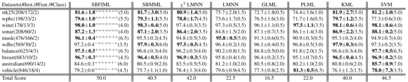
Table 1.Mean and standard deviation of 5 times 10-fold CV accuracy results onRddatasets. The superscripts+−=next to the accuracies
of SBFIML indicate the result of the Student’s t-test with SBMML,χ2 LMNN, LMNN, GLML, PLML, KML and SVM. They denote respectively a significant win, loss or no difference for SBFIML. Theboldentries for each dataset have no significant difference from the best accuracy for that dataset. The number in the parenthesis indicates the score of the respective algorithm for the given dataset based on the pairwise comparisons of the Student’s t-test.
Datasets(#Inst./#Feat./#Class) SBFIML SBMML χ2LMNN LMNN GLML PLML KML SVM stk25(208/172/2) 81.6±1.8==+++==(5.0) 81.7±3.0(5.0) 80.9±1.4(5.0) 75.7±2.0(1.5) 72.7±1.8(0.5) 74.4±3.6(1.0) 81.9±2.7(5.0) 81.2±1.0(5.0) wpbc(198/33/2) 79.6±1.0==+++=+(5.5) 79.3±1.1(5.5) 78.8±1.7(4.5) 73.6±1.7(0.5) 76.5±1.6(3.0) 71.7±1.6(0.5) 79.7±1.2(5.5) 77.3±0.6(3.0) wine(178/13/3) 98.0±1.0===+===(4.0) 98.3±0.4(5.0) 97.4±0.3(3.5) 97.3±0.5(3.5) 96.1±1.1(0.5) 97.5±1.1(3.5) 98.1±0.6(4.0) 98.1±0.6(4.0) sonar(208/60/2) 87.2±1.3==+====(4.0) 87.1±2.0(3.5) 86.4±2.0(3.5) 84.8±1.5(2.0) 87.1±0.7(3.5) 86.1±1.4(3.0) 86.9±2.2(3.5) 88.1±0.2(5.0) musk(476/166/2) 96.1±0.4++=++++(6.5) 95.5±0.2(4.5) 94.8±0.5(3.0) 95.8±0.5(5.0) 91.3±0.6(0.5) 90.9±0.3(0.5) 95.3±0.2(4.0) 94.9±0.7(4.0) wdbc(569/30/2) 97.2±0.4−=++=−=(3.5) 97.9±0.3(6.0) 97.5±0.5(4.5) 96.4±0.2(1.0) 96.1±0.4(0.5) 96.8±0.5(3.0) 97.9±0.3(6.0) 97.3±0.2(3.5) balance(625/4/3) 97.5±0.5++++++=(6.5) 96.6±0.3(4.0) 96.2±0.5(4.0) 90.2±0.8(1.5) 88.8±0.5(0.0) 91.8±2.0(1.5) 96.6±0.3(4.0) 97.7±0.5(6.5) breast(683/10/2) 96.7±0.3==+=+==(4.5) 96.4±0.5(4.0) 96.9±0.3(5.0) 95.8±0.4(1.0) 96.4±0.2(3.5) 95.1±0.7(0.5) 96.5±0.4(4.5) 96.9±0.2(5.0) australian(690/14/2) 84.6±0.3++++++−(6.0) 80.5±0.9(2.0) 83.5±0.5(5.0) 81.2±1.0(2.0) 80.5±0.8(2.0) 80.2±1.0(2.0) 80.8±0.6(2.0) 85.7±0.9(7.0) vehicle(846/18/4) 79.2±0.6+==+−+=(4.5) 75.7±1.1(1.0) 78.4±1.3(4.0) 79.6±0.9(4.5) 77.3±0.8(2.5) 81.3±0.5(6.5) 76.1±1.2(1.5) 78.0±7.3(3.5) Total Score 50.0 40.5 42.0 22.5 16.5 22.0 40.0 46.5
SBFIML against three metric learning baseline methods: LMNN (Weinberger & Saul,2009)2, KML (Wang et al.,
2011)3, GLML (Noh et al.,2009), and PLML (Wang et al.,
2012). The former two learn a global Mahalanobis metric
in the input feature spaceRdand the RKHS space
respec-tively, and the last two learn smooth local metrics in Rd.
In addition, we also compare SBFIML against Similarity-based Mahalanobis Metric Learning (SBMML) to see the difference of pullback metrics G∗Q(x), equation 10, and
G∗P(x), equation 11. SBMML learns a global
Maha-lanobis metric in the proximity space Q. Similar to
SB-FIML, the metric is learned by optimizing the problem16,
in which the cosine distance is replaced by Mahalanobis
distance. The constraints onLin problem16are also
re-moved. To see the difference between the cosine distance
used in SBFIML and theχ2distance used inχ2LMNN,
we compare SBFIML againstχ2LMNN. Note that, both
methods solve exactly the same optimization problem16
but with different distance computations. Finally, we also compare SBFIML against SVM for binary classification problems and against multi-class SVMs for multiclass clas-sification problems. In multi-class SVMs, we use the one-against-all strategy to determine the class label.
KML, SBMML andχ2LMNN learn an×nPSD matrix
and are thus computationally expensive for datasets with large number of instances. To speedup the learning process, similar to SBFIML, we can learn a low rank transformation
matrixLof sizek×n. For all methods, KML, SBMML,
χ2LMNN and SBFMIL, we set k = 0.1nin all
experi-ments. The matrixLin KML and SBMML was initialized
by clipping then×nidentity matrix into the size ofk×n.
In a similar manner, inχ2LMNN and SBFIML the matrix
Lwas initialized by applying on the initialization matrixL
in KML a simplex projector which ensures the constraints in problem (16) are satisfied.
The LMNN has one hyper-parameter µ (Weinberger &
2
http://www.cse.wustl.edu/∼kilian/code/code.html. 3http://cui.unige.ch/∼wangjun/.
Saul, 2009). We set it to its default value µ = 1. As
in (Noh et al., 2009), GLML uses the Gaussian distri-bution to model the learning instances of a given class.
The hyper-parameters of PLML was set following (Wang
et al., 2012). The SBFIML has two hyper-parameters α
andγ. Following LMNN (Weinberger & Saul,2009), we
set theαparameter to1. We select the margin parameterγ
from{0.0001,0.001,0.01,0.1}using a 4-fold inner Cross Validation (CV). The selection of an appropriate similarity function is crucial for SBFIML. We choose the similarity function with a 4-fold inner CV from the angular similarity, equation (8), and the Gaussian similarity in equation (7). We examine two types of Gaussian similarity. In the first we set allσk toσwhich is selected from{0.5τ, τ,2τ},τ
was set to the average of all pairwise distances. In the
sec-ond we set theσkfor each anchor pointzkseparately; the
σkwas set by making the entropy of the conditional
distri-butionp(xi|zk) =
sk(xi)
Pn
i=1sk(xi)equal tolog(nc)(Hinton &
Roweis,2002), wherenis the number of training instances andcwas selected from{0.8,0.9,0.95}.
Since χ2 LMNN and SBFIML apply different distance
parametrizations to solve the same optimization problem,
the parameters ofχ2 LMNN are set in exactly the same
way as SBFIML, except that the margin parameter γ of
χ2 LMNN was selected from {10−8,10−6,10−4,10−2},
because χ2 LMNN uses the squaredχ2distance (Kedem
et al.,2012). The best similarity map forχ2LMNN is also
selected using a 4-fold inner CV from the same similarity function set as that of SBFIML.
Akin to SBFIML, the performance of KML and SVM de-pends heavily on the selection of the kernel. We select au-tomatically the best kernel with a 4-fold inner CV. The ker-nels are chosen from the linear, the set of polynomial (de-gree 2,3 and 4), the angular similarity, equation (8), and the
Gaussian kernels with widths{0.5τ, τ,2τ}, as in SBFIML
τ was set to the average of all pairwise distances. In
addi-tion, we also select the margin parameterγof KML from
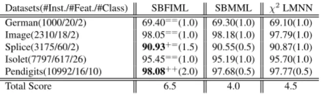
se-Table 2.Accuracy results on large datasets. Datasets(#Inst./#Feat./#Class) SBFIML SBMML χ2LMNN German(1000/20/2) 69.40==(1.0) 69.30(1.0) 69.10(1.0) Image(2310/18/2) 98.05==(1.0) 98.18(1.0) 97.79(1.0) Splice(3175/60/2) 90.93+=(1.5) 90.55(0.5) 90.87(1.0) Isolet(7797/617/26) 95.45==(1.0) 95.19(1.0) 95.70(1.0) Pendigits(10992/16/10) 98.08++(2.0) 97.68(0.5) 97.77(0.5) Total Score 6.5 4.0 4.5
lected from{0.01,0.1,1,10,100}. SBMML does not have
any constraints on the similarity function, thus we select its similarity function with a 4-fold inner CV from a set which includes all kernel and similarity functions used in SBFIML and KML. As in KML, we select the margin
pa-rameterγof SBMML from{0.01,0.1,1,10,100}. For all
methods, except GLML and SVM which do not involve triplet constraints, the triplet constraints are constructed us-ing three same-class and ten different-class nearest neigh-bors for each learning instance. Finally, we use the 1-NN rule to evaluate the performance of the different metric learning methods.
To estimate the classification accuracy we used 5 times 10-fold CV. The statistical significance of the differences were tested using Student’s t-test with a p-value of 0.05. In order to get a better understanding of the relative performance of the different algorithms for a given dataset we used a sim-ple ranking schema in which an algorithm A was assigned one point if it was found to have a statistically significantly better accuracy than another algorithm B, 0.5 points if the two algorithms did not have a significant difference, and zero points if A was found to be significantly worse than B.
Results. In Table1we report the accuracy results. We see that SBFIML outperforms in a statistical significant man-ner the single metric learning method LMNN and the local metric learning methods, GLML and PLML, in seven, eight and six out of ten datasets respectively. When we compare it to KML and SBMML, which learn a Mahalanobis met-ric in the RKHS and proximity space, respectively, we see that it is significantly better than KML and SBMML in four datasets and significantly worse in one dataset. Compared
toχ2 LMNN, SBFIML outperformsχ2-LMNN on eight
datasets, being statistically significant better on three, and it never loses in statistical significant manner. Finally, com-pared to SVM, we see that SBFIML is significantly better in two datasets and significantly worse in one dataset. In terms of the total score, SBFIML achieves the best predic-tive performance with 50 point, followed by SVM ,which
scores 46.5 point, andχ2-LMNN with 42 point. The local
metric learning method GLML is the one that performs the worst. A potential explanation for the poor performance of GLML could be that its Gaussian distribution assumption is not that appropriate for the datasets we experimented with. To provide a better understanding of the predictive
per-formance difference between SBFIML, SBMML, andχ2
LMNN, we applied them on five large datasets. To speedup
the learning process, we use as anchor points20%of
ran-domly selected training instances. Moreover, the
param-eter k of low rank transformation matrix L was reduced
tok = 0.05n, where nis the number of anchor points. The kernel function and similarity map was selected using 4-fold inner CV. The classification accuracy of Isolet and Pendigits are estimated by the default train and test split, for other three datasets we used 10-fold cross-validation. The statistical significance of difference were tested with McNemar’s test with p-value of 0.05.
The accuracy results are reported in Table 2. We see
that SBFIML achieves statistical significant better accuracy than SBMML on the two datasets, Splice and Pendigits.
When compare it toχ2LMNN, we see it is statistical
sig-nificant better on one dataset, Pendigits. In terms of
to-tal score, SBFIML achieves the best score,6.5points,
fol-lowed byχ2LMNN.
5. Conclusion
In this paper we present a two-stage metric learning al-gorithm SBFIML. It first maps learning instances onto a statistical manifold via a similarity-based differential map and then defines the distance in the input data space by the Fisher information distance on the statistical manifold. This induces a new family of distance metrics in the input data space with two important properties. First, the induced metrics are robust to density variations in the original data space and second they have largest distance discrimina-tion on the manifold of the anchor points. Furthermore, by learning a metric on the statistical manifold SBFIML can learn distances on different types of input feature spaces. The similarity-based map used in SBFIML is natural and flexible; unlike KML it does not need to be PSD. In addi-tion SBFIML can be interpreted as a local metric learning method with a well defined distance approximation. The experimental results show that it outperforms in a statis-tical significant manner both metric learning methods and SVM.
Acknowledgments
Jun Wang was partially funded by the Swiss NSF (Grant 200021-122283/1). Ke Sun is partially supported by the Swiss State Secretariat for Education, Research and In-novation (SER grant number C11.0043). Fei Sha is sup-ported by DARPA Award #D11AP00278 and ARO Award #W911NF-12-1-0241
References
Amari, S. and Cichocki, A. Information geometry of
di-vergence functions. Bulletin of the Polish Academy of
Sciences: Technical Sciences, 58(1):183–195, 2010.
Amari, S. and Nagaoka, H. Methods of information
geom-etry, volume 191. Amer Mathematical Society, 2007.
Chen, Jianhui and Ye, Jieping. Training svm with indefinite
kernels. InProceedings of the 25th international
confer-ence on Machine learning, pp. 136–143. ACM, 2008. Chen, Yihua, Garcia, Eric K., Gupta, Maya R., Rahimi,
Ali, and Cazzanti, Luca. Similarity-based classification:
Concepts and algorithms. JMLR, 2009.
Cuturi, M. and Avis, D. Ground metric learning. arXiv
preprint arXiv:1110.2306, 2011.
Davis, J.V., Kulis, B., Jain, P., Sra, S., and Dhillon, I.S.
Information-theoretic metric learning. InICML, 2007.
Duchi, J., Shalev-Shwartz, S., Singer, Y., and Chandra, T. Efficient projections onto the l 1-ball for learning in high
dimensions. InICML, 2008.
Hauberg, Sren, Freifeld, Oren, and Black, Michael. A ge-ometric take on metric learning. In Bartlett, P., Pereira, F.C.N., Burges, C.J.C., Bottou, L., and Weinberger, K.Q.
(eds.),Advances in Neural Information Processing
Sys-tems 25, pp. 2033–2041, 2012.
Hinton, G. and Roweis, S. Stochastic neighbor embedding.
Advances in neural information processing systems, 15: 833–840, 2002.
Honeine, P. and Richard, C. The angular kernel in machine
learning for hyperspectral data classification. In
Hyper-spectral Image and Signal Processing: Evolution in Re-mote Sensing (WHISPERS), 2010 2nd Workshop on, pp. 1–4. IEEE, 2010.
Jain, P., Kulis, B., and Dhillon, I. Inductive regularized
learning of kernel functions. Advances in Neural
Infor-mation Processing Systems, 23:946–954, 2010.
Kass, R.E. and Vos, P.W. Geometrical foundations of
asymptotic inference, volume 908. Wiley-Interscience, 2011.
Kedem, Dor, Tyree, Stephen, Weinberger, Kilian, Sha, Fei,
and Lanckriet, Gert. Non-linear metric learning. In
Bartlett, P., Pereira, F.C.N., Burges, C.J.C., Bottou, L.,
and Weinberger, K.Q. (eds.),Advances in Neural
Infor-mation Processing Systems 25, pp. 2582–2590, 2012.
Lebanon, G. Metric learning for text documents. Pattern
Analysis and Machine Intelligence, IEEE Transactions
on, 28(4):497–508, 2006.
Lee, J.M. Introduction to smooth manifolds, volume 218.
Springer, 2002.
Lee, S.M., Abbott, A.L., and Araman, P.A.
Dimen-sionality reduction and clustering on statistical
mani-folds. In Computer Vision and Pattern Recognition,
2007. CVPR’07. IEEE Conference on, pp. 1–7. IEEE, 2007.
Noh, Y.K., Zhang, B.T., and Lee, D.D. Generative local metric learning for nearest neighbor classification.NIPS, 2009.
Radhakrishna Rao, C. Information and accuracy attainable in the estimation of statistical parameters.Bulletin of the Calcutta Mathematical Society, 37(3):81–91, 1945. Van der Maaten, Laurens and Hinton, Geoffrey. Visualizing
data using t-sne.Journal of Machine Learning Research,
9(2579-2605):85, 2008.
Wang, J., Do, H., Woznica, A., and Kalousis, A. Metric
learning with multiple kernels. Advances in Neural
In-formation Processing Systems. MIT Press, 2011. Wang, Jun, Kalousis, Alexandros, and Woznica, Adam.
Parametric local metric learning for nearest neighbor classification. In Bartlett, P., Pereira, F.C.N., Burges,
C.J.C., Bottou, L., and Weinberger, K.Q. (eds.),
Ad-vances in Neural Information Processing Systems 25, pp. 1610–1618, 2012.
Weinberger, K.Q. and Saul, L.K. Distance metric
learn-ing for large margin nearest neighbor classification. The
Journal of Machine Learning Research, 10:207–244, 2009.
Ying, Y., Campbell, C., and Girolami, M. Analysis of svm
with indefinite kernels. Advances in Neural Information