Bayesian Methods and Machine Learning in Astrophysics

(1)

Bayesian Methods and

Machine Learning in

Astrophysics

Edward John Higson Cavendish Astrophysics Group

Gonville & Caius College 1st October 2018

A dissertation submitted for the degree of Doctor of Philosophy at the University of Cambridge

(2)

(3)

Declaration

This dissertation is the result of my own work and includes nothing which is the outcome of work done in collaboration except as declared in the Preface and specified in the text.

The use of “we” is a stylistic choice.

It is not substantially the same as any that I have submitted, or, is being concurrently submitted for a degree or diploma or other qualification at the University of Cambridge or any other University or similar institution except as declared in the Preface and specified in the text. I further state that no substantial part of my dissertation has already been submitted, or, is being concurrently submitted for any such degree, diploma or other qualification at the University of Cambridge or any other University or similar institution except as declared in the Preface and specified in the text.

It does not exceed the prescribed word limit for the relevant Degree Committee (60,000 words).

Much of the material in this thesis has also been presented in Higson et al. (2018, 2019a,b,c); this work was done in collaboration with the candidate’s supervisors (An-thony Lasenby, Mike Hobson and Will Handley).

(4)

(5)

Acknowledgements

I am extremely grateful to Anthony Lasenby and Mike Hobson for all their help and guidance over the last 3 years. I could not have wished for better supervisors; it has been a privilege working with them and I have learned an immense amount from the experience. I am equally grateful to Will Handley for his triple role in my PhD — as a third supervisor, a perennial code fixer and a friend.

I would also like to take this opportunity to thank the many people who inspired and fed my interest in physics and research over my many years in education. This includes (but is by no means limited to) David Wolfe and Anton Machacek at the Royal Grammar School High Wycombe, Peter Norreys and Raoul Trines at the Rutherford Appleton Laboratory, and Tony Weidberg, Georg Viehhauser, Devinder Sivia, Andrei Starinets and Ralph Sch¨onrich at Oxford University.

I am grateful to my officemates Bjoern Soergel, Carina Negreanu, Iulia Simion, Fruzsina Agocs, Lukas Hergt and Pablo Lemos-Portela for their help with (and distrac-tion from) various research challenges. Special thanks also goes to my fellow Cambridge-based expatriates from The Other Place — Jack Anthony, Jacob Swain and Peter Taylor — for their proof-reading services.

Most importantly I thank my loving parents, Jackie and Mark, for all the unwavering support (financial, emotional and logistical) they have provided throughout my life.

I dedicate this thesis to Harriet Smith, who has put up with me for 9 years now and I hope will continue to do so.

(6)

(7)

Summary

This thesis is concerned with methods for Bayesian inference and their applications in astrophysics. We principally discuss two related themes: advances in nested sam-pling (Chapters 3 to 5), and Bayesian sparse reconstruction of signals from noisy data (Chapters 6 and 7).

Nested sampling is a popular method for Bayesian computation which is widely used in astrophysics. Following the introduction and background material in Chapters 1 and 2, Chapter 3 analyses the sampling errors in nested sampling parameter estimation and presents a method for estimating them numerically for a single nested sampling calculation (this was published in Higson et al., 2018). Chapter 4 introduces diagnostic tests for detecting when software has not performed the nested sampling algorithm accurately, for example due to missing a mode in a multimodal posterior, and uses material from Higson et al. (2019b). The uncertainty estimates and diagnostics in Chapters 3 and 4 are implemented in thenestcheck (Higson, 2018b) software package. Chapter 5, presented in Higson et al. (2019a), describes dynamic nested sampling: a generalisation of the nested sampling algorithm which can produce large improvements in computational efficiency compared to standard nested sampling. We have imple-mented dynamic nested sampling in the dyPolyChord (Higson, 2018a) andperfectns

(Higson, 2018c) software packages.

Chapter 6 presents a principled Bayesian framework for signal reconstruction, in which the signal is modelled by basis functions whose number (and form, if required) is determined by the data themselves. This approach is based on a Bayesian interpretation of conventional sparse reconstruction and regularisation techniques, in which sparsity is imposed through priors via Bayesian model selection. We demonstrate our method for noisy 1- and 2-dimensional signals, including examples of processing astronomical images. The numerical implementation uses dynamic nested sampling, and uncertainties

(8)

are calculated using the methods introduced in Chapters 3 and 4. Chapter 7 applies our Bayesian sparse reconstruction framework to artificial neural networks, where it allows the optimum network architecture to be determined by treating the number of nodes and hidden layers as parameters. Chapters 6 and 7 use material from Higson et al. (2019c).

(9)

Introduction

As astrophysicists, we aim to create theories which describe the natural phenomena we observe in the universe. The scientific method requires that we test our hypotheses empirically; this allows them to be falsified or refined, and enables us to choose between rival models. Consequently, making inferences from data is fundamental to the research process.

This empirical scientific method is not new; a detailed account can be found in Sir Francis Bacon’s 1620 workNovum Organum Scientiarum (“New Instrument of Sci-ence”). However, modern advances in experiments and computing have made data analysis techniques more important to scientific research now than ever before. In as-trophysics in particular, the last two decades have seen order-of-magnitude increases in the quantity of both data and computational resources available. This has revolu-tionised our understanding of many aspects of the universe, and made advances in data analysis techniques and numerical methods central to the progress of the field.

The first theme of this thesis, advances in nested sampling, contributes to solving the challenges posed by these recent increases in the size and complexity of astronomical data. After a review of Bayesian inference methods and theory in Chapter 2, Chapters 3 and 4 provide practical tools for assessing the uncertainty and reliability of nested sam-pling calculations — which are poorly understood compared to many other numerical methods. Such calculations underpin a large number of recent results in astrophysics, but their reliability is not guaranteed; properly checking results is therefore of great scientific importance. Astronomical applications of the techniques introduced can be found in Sections 3.7 and 4.7.

(14)

Chapter 5 introduces dynamic nested sampling: a new algorithm which can pro-vide order-of-magnitude improvements in computational efficiency over standard nested sampling, permitting the analysis of larger and more complex data sets. Since the pub-lication of the dynamic nested sampling algorithm, its apppub-lications in astronomy have included constraining the present day stellar mass function (Orazio et al., 2018), fitting light curves of transient sources (Guillochon et al., 2018) and mapping distances across the Perseus molecular cloud (Zucker et al., 2018).

The thesis’ second theme, Bayesian sparse reconstruction of signals, introduces a principled approach for fitting data using machine learning techniques such as regres-sion1 and neural networks. In Chapter 6 we describe our Bayesian sparse reconstruction framework, in which signals are fitted using basis functions whose number (and, if re-quired, form) is determined by the data themselves. We show that this can be done by treating the type and number of basis functions as integer parameters, then per-forming Bayesian model selection indirectly by sampling the posterior distribution of these parameters. Chapter 7 applies this approach to artificial neural networks, where it allows Bayesian model selection to be performed over the space of possible network architectures by treating the number of hidden layers and nodes as integer parameters. Demonstrations of our method in Chapters 6 and 7 include applications to processing astronomical images.

Our Bayesian sparse reconstruction research is closely linked to recent advances in computing power and numerical methods such as nested sampling, which have made this principled approach feasible in the low data regime. We also make use of diagnostic tests and the dynamic nested sampling algorithm, introduced in Chapters 3 to 5, in the numerical calculations in Chapters 6 and 7. We intend the examples of Bayesian sparse reconstruction in this thesis to serve as a proof of principle for a wider range of astronomical applications, which will be made possible by future improvements in computational hardware and numerical methods.

1_{The modern field of “machine learning” incorporates a number of classical statistical techniques}

which significantly predate the coining of the term by Arthur Samuel in the 1950s. This includes regression, the earliest form of which dates back to Legendre (1805).

(15)

Chapter 2

Bayesian inference

We now provide an overview of Bayesian inference, which is central to the work in subsequent chapters of this thesis. Many excellent books on this topic exist; in particular we use Sivia and Skilling (2006) and MacKay (2003). In addition there are some good review articles on Bayesian methods in the context of astrophysics and cosmology; we have drawn from Trotta (2008), Loredo (2012) and Sharma (2017). The chapter finishes with an introduction to nested sampling in Section 2.4, which will provide background for Chapters 3 to 5. Some sections of this chapter have been adapted from background material presented in Higson et al. (2018, 2019c).

2.1 Bayesians and frequentists

We first introduce Bayesian inference by contrasting it with the rival frequentist paradigm.

2.1.1 Probability

The distinction between Bayesians and frequentists can be understood in terms of the two schools’ differing definitions of probability. A frequentist definition is:

“Probability is an event’s relative frequency in the limit of an infinite number of independent trials.”

At first glance this definition makes intuitive sense, but it has a number of significant shortcomings identified by Trotta (2008). These include:

(16)

1. it cannot formulate perfectly reasonable questions involving unrepeatable events. For example, “what is the probability that King Richard III arranged the murder of his two young nephews (the princes in the tower) in 1483?”;

2. to hold exactly it requires an infinite number of trials, which are never available in practice. Small sample sizes requiread hoc and potentially complex adjustments; 3. it is circular, in that it assumes the event has the same probability of occurring in

each trial when this probability is exactly what we seek to define;

4. it covers only random processes (aleatoric uncertainty), such as the probability of an atomic nucleus undergoing radioactive decay within some time period. Epis-temic uncertainty due to a lack of knowledge about a deterministic system is not included.

As a consequence, this definition of “probability” is often radically different to the word’s meaning when it is used colloquially. Imagine you suggest to your friend that you leave a cake in the oven for 45 minutes to bake, and they reply “if we do that, there is a 50% probability we will burn it!” Does your friend mean to tell you that, if you left a very large number of identical cakes in identical ovens at identical temperatures for 45 minutes, approximately half of them would be burned and half of them not burned? This seems somewhat unlikely. More plausibly, rather than suggesting the baking process is stochastic, your friend believes it is broadly deterministic but is unsure of the outcome. In such a conversation we implicitly assume a Bayesian definition of probability, which does not suffer from the problems with the frequentist version identified above:

“Probability is a measure of the degree of belief that a proposition is true.”

This definition is not circular, and can clearly be applied to unrepeatable events and limited numbers of samples. Furthermore, it does not distinguish between uncertainty due to a process’ intrinsic randomness and due to lack of information.

2.1.2 Bayes’ theorem

In order to use the Bayesian definition of probability to analyse new data, we require a method for updating our degree of belief in a proposition given new information. The mathematical formula for this procedure is credited to the Reverend Thomas Bayes

(17)

(1701(?)-1761), from whom Bayesian statistics takes its name. Bayes’ eponymous the-orem was published posthumously in 1763, by his friend the philosopher Richard Price (Bayes and Price, 1763).

Bayes’ theorem can be derived from the axioms required for consistent reasoning (the “Cox axioms”), which imply that the probabilities of propositions X and Y must satisfy the sum and product rules (Sivia and Skilling, 2006). The sum rule states

P(X|I) +P( ¯X|I) = 1, (2.1)

where ¯X denotes “not X” and P(X|I) ∈ [0,1]. Here P(X|I) denotes the conditional probability of X given I, and following Sivia and Skilling (2006) we explicitly include that all probabilities are conditional on any background informationI. Such conditional probabilities represent logical rather than causal or temporal connections; for example future events can provide us with more information about the probabilities of past events. The product rule is

P(X, Y_|I) =P(X_|Y, I)P(Y_|I). (2.2)

Bayes’ theorem can be easily derived from (2.2) by noting P(X, Y_|I) =P(Y, X_|I), so

P(X|Y, I)P(Y|I) =P(Y|X, I)P(X|I), (2.3)

and hence

P(X_|Y, I) = P(Y|X, I)P(X|I)

P(Y|I) . (2.4)

This provides a formula for updating our prior degree of belief P(X_|I), termed the

prior, with new information Y. It is worth mentioning that Bayes’ theorem is an uncontroversial mathematical statement, and the disagreement between Bayesians and frequentists is about its use as a basis for inference (Trotta, 2008).

Until this point we have focused on “propositions” X and Y which can be true or false, but Bayes’ theorem (2.4) and the Bayesian definition of probability also extend to quantities which can take a range of discrete or continuous values. In the discrete case

X takes values in [X1, X2, . . .], and the sum rule (2.1) becomes

X

i

(18)

whereP(Xi|I)∈[0,1] for alli. In the continuous caseX takes values in Rand Z ∞

−∞

P(X|I) dX= 1, (2.6)

where P(X|I) > 0 for all X ∈ R. Another significant result which follows from the

Cox axioms is “marginalisation” (also called the “law of total probability”), which for continuous variables X and Y can be written as

P(X|I) =

Z ∞

−∞

P(X, Y|I) dY. (2.7)

This allows the removal (“marginalising out”) of parameters from joint distributions, and is of great importance for Bayesian inference. We use the notation in this section for the remainder of this thesis, although more rigorous conventions are common in the statistics literature.

2.1.3 Practical differences

Perhaps the most commonly cited difference between the Bayesian and frequentist ap-proaches is the former’s requirement that the initial knowledge of the proposition is specified mathematically in the prior. This introduces additional subjectivity and com-plexity, and is often viewed by non-Bayesians as a disadvantage. Indeed simply specify-ing an absence of knowledge — a non-informative prior — often requires careful analysis (for some examples see Handley and Millea, 2018; Sivia and Skilling, 2006). However it can be argued that the inclusion of the prior is not a limitation but a feature of the Bayesian approach (Trotta, 2008), as it serves to make assumptions explicit and to model the fact that different scientists can interpret the same data differently given their distinct previous experiences. In addition there are many circumstances when there is an uncontroversial basis for the inclusion of prior information, such as when analysing noisy measurements of a physical variable that we know must be positive or take a value within some range.

We take the view of Loredo (2012), who argues the most fundamental difference between calculations using the two approaches is not the modulation by the prior but the space over which the analysis takes place. Whereas a frequentist calculation takes place in the sample space (the space of possible measurements), Bayesian computation is performed in the parameter (hypothesis) space. This perspective elucidates the necessity

(19)

of the prior to provide a measure over the parameter space to be analysed. If the prior were not included, inferences about some physical quantity involving averaging it (integrating its distribution over the parameter space) could be affected by simple reparameterisations; for an interesting discussion of this see Loredo (2012, p10-12). The exploration of the parameter space is a key aspect of the Bayesian computation techniques discussed in Section 2.3.

2.1.4 Why isn’t everyone a Bayesian?

Given the philosophical advantages of the Bayesian approach discussed in Section 2.1.1 and the persuasive arguments presented by Trotta (2008), Sivia and Skilling (2006) and Loredo (2012) among others, it is reasonable to ask why everyone is not a Bayesian. In fact, historically, most 19th century scientists used a Bayesian perspective, including notably Laplace — who derived Bayes’ theorem independently and first expressed it in its modern form (2.4) (Sivia and Skilling, 2006).

This changed in the 20th century with the introduction of two successful rival fre-quentist frameworks: Fisher’s “significance testing” and Neyman-Pearson “hypothesis testing”. These approaches introduce a variety of procedures without a clear overarch-ing rationale (Sivia and Skilloverarch-ing, 2006). However they claim the advantages of ease of application and objectivity, in particular in comparison to the careful thought1 often needed to choose the priors in a Bayesian analysis; interesting discussions can be found in Efron (1986) and Gelman (2008).

Unsurprisingly many Bayesians dispute these claims, including Loredo (2012) and Sivia and Skilling (2006). Furthermore frequentist statistics can also lead to subtle problems when not used carefully, withp-value significance tests believed to be a major cause of the “replication crisis” currently being experienced in the social sciences (for more details see the recent American Statistical Association statement by Wasserstein and Lazar, 2016). We are currently seeing rapid growth in the popularity of Bayesian methods, in particular in astrophysics, and many predict the 21st _{century will see a}

return to the dominance of the Bayesian school (Loredo, 2012; Lindley, 1975). However, the debate is far from settled (Trotta, 2008).

1_{Gelman (2008), writing in the voice of a hypothetical anti-Bayesian, quips that “recommending}

(20)

Having provided some context, the remainder of this chapter and this thesis will now focus on the Bayesian approach.

2.2 Applying Bayes’ theorem to data

Scientific research is about creating models to explain and understand available data. Models and their parameters offer a description of the universe, which we use to work out how likely we are to observe a given set of data values. However, as scientists our primary goal is to solve the inverse problem — i.e. make an inference about the state of the universe (which model is correct, and what are the model’s parameter values) given the data. Such inferences can be divided intoparameter estimationandmodel selection. Given some model M, parameter estimation involves determining the values of its parameters θ using the data D. Bayes’ theorem (2.4) can be applied to parameter estimation by replacingI with the modelM,X with the model’s parametersθ andY

with the data D. This gives

P(θ_|D,_M) = P(D|θ,M)P(θ|M)

P(_D|M) , (2.8)

which we write schematically as

P(θ) = L(θ)π(θ)

Z . (2.9)

Here the prior

π(θ)_≡P(θ_|M) (2.10)

represents our knowledge of the model’s parameters in the absence of the data. The model tells the probability of observing data D given some set of parameter values θ, and can therefore be expressed as a distributionP(D|θ,M) which we term thelikelihood

and write as

L(θ)≡P(D|θ,M). (2.11)

Thus Bayes’ theorem allows us to update our prior knowledgeπ(θ) given new informa-tion _Dto obtain theposterior distribution

(21)

|logBjk| Odds Notes

<1.0 /3 : 1 Inconclusive

1.0 ≈3 : 1 Positive evidence

2.5 _≈12 : 1 Moderate evidence

5.0 _≈150 : 1 Strong evidence

Table 2.1: The “Jeffreys’ scale” for interpreting the Bayes factor between two models Mj and Mk, reproduced from Trotta (2007). The first column shows the log Bayes factor value, the second column shows the approximate relative odds of the two models being correct and the third column gives a qualitative interpretation.

The Bayesian evidence _Z is a normalisation constant, and is computed by averaging the likelihood _L(θ) over the priorπ(θ)

Z ≡P(_D|M) =

Z

L(θ)π(θ) dθ. (2.13)

Bayes’ theorem can also be used to compare different models_M1,M2, . . . and assess

which best describes the data. The posterior probability of a given model is

P(_Mj|D) = P(D|Mj)P(Mj) P(_D) = ZjΠj P kZkΠk , (2.14)

where Πj ≡P(Mj) denotes the prior probability of each model and the denominator of the final term sums over all competing models. The evidence Z penalises more complex models so this approach naturally includes Occam’s razor. Models may also be compared by computing log posterior odds ratios

Pkj ≡log P(_Mj|D) P(Mk|D) = log Zj Zk + log Πj Πk , (2.15)

where here and in the remainder of this thesis log denotes the natural logarithm. The ratio of evidences_Bj_k=_Zj/Zkis called a Bayes factor; Bayes factors are independent of the prior Πj on different modelsMj, but depend on the priors on the models’ parameters

π(θ_M_j) through the calculation of_Zj from (2.13). If the prior Πj on different models is uniform, the Bayes factors are equal to the posterior odds ratios. The “Jeffreys’ scale” (Jeffreys, 1961) provides a numerically calibrated scale for qualitatively interpreting Bayes factors; we reproduce a modified version from Trotta (2007) in Table 2.1.

(22)

2.3 Bayesian computation

In some simple cases, parameter estimation (2.9) and model comparison (2.14) calcula-tions can be performed analytically. However for most problems in astronomy this is not possible, and numerical calculations are required. One technique for doing this isnested sampling, which is a major focus of this thesis. This section provides an overview of some Bayesian computation techniques which are popular in astrophysics, in order to provide context for our discussion of nested sampling in Section 2.4. Many excellent guides to this topic are available; we have used Sharma (2017), Hogg and Foreman-Mackey (2018) and Feroz (2008).

Likelihoods _L(θ) are often computationally expensive functions, so the goal of Bayesian computation is to obtain posterior inferences using a limited number of eval-uations of the likelihood function (“likelihood calls”). The number of likelihood calls required for numerical integration (for example by quadrature) increases exponentially with the dimensionality of the parameter space, so this approach is typically impractical except in very low dimensions. As a result Bayesian computation is usually carried out using Monte Carlo methods, which involve repeated random sampling.

2.3.1 Parameter estimation

Parameter estimation calculations can be performed by generating a set of samples from the posterior distribution, then using these to make inferences about quantities of interest such as the posterior means of parameters. Samples can also be used to numerically estimate the posterior distributions of parameters or functions of parameters with kernel density estimation.

In astronomy the most popular approach for generating samples is to use Markov chain Monte Carlo (MCMC); a class of methods for sampling probability distributions which explore the parameter space via a biased random walk (Hogg and Foreman-Mackey, 2018). Samples produced by these methods form a Markov chain, meaning that the probability distribution of the next random variableθi+1 depends only on the

current stateθi and is independent of the previous evolution of the sequence. The chains should have the property that, after a large number of steps from the starting point, the samples produced will have an invariant limiting distribution which is proportional to the posterior distribution (hence the chains must be ergodic). This can be achieved if

(23)

the rule for selecting a new point satisfies certain conditions (see Sharma, 2017; MacKay, 2003, for a detailed discussion). Most MCMC methods satisfydetailed balance, meaning that the probability of being in one state and transitioning to another state is the same in either direction and as a result the process is reversible.

The Metropolis-Hastings algorithm (Metropolis et al., 1953; Hastings, 1970) is the most general MCMC algorithm (Sharma, 2017), and is shown in Algorithm 1. New points are added via a two step process: first a candidate point is sampled from a proposal distribution q(θ0_|θi), then it is accepted or rejected with a probability which depends on the value of the posterior at the candidate point P(θ0) relative to the pos-terior at the previous point P(θi). Most variants use symmetric proposal distribu-tions which satisfy q(θ0|θi) = q(θi|θ0); this simplifies the condition for acceptance to

U < P(θ0)/P(θi) (where U ∈ [0,1] is a uniform random variable). In this case, if

P(θ0)>P(θi) then the candidate point is guaranteed to be accepted — but it may be rejected otherwise. This biases the random walk towards regions whereP(θ) is high, and is the mechanism by which the distribution of samples produced is made proportional toP(θ).

Result: Samples _{θi} from the posteriorP(θ).

Input: Posterior distribution function_P(θ), starting pointθ1, proposal

distributionq(θ0|θi).

for i= 1 to N₋1do

sample θ0 from q(θ0_|θi);

sample uniform random variable U ∈[0,1];

if U < P(θ0)q(θi|θ0) P(θi)q(θ0|θi) then θi+1 =θ0; else θi+1 =θi; end end

Algorithm 1:The Metropolis-Hastings algorithm.

There are many variants of the Metropolis-Hastings approach (Algorithm 1). These include:

Gibbs sampling: different parameters (components of θ) are updated individually using sampling from conditional distributions (Geman and Geman, 1984). Unlike in Algorithm 1, all samples are accepted.

(24)

Adaptive MCMC: the proposal distribution is dynamically adapted based on past samples (see Andrieu and Thoms, 2008, for a review).

Affine invariant ensemble samplers: an ensemble of interacting Markov chains is used, and the resulting process’ performance is unaffected by affine transforma-tions of the parameter space (Goodman and Weare, 2010). The popular emcee

package (Foreman-Mackey et al., 2013) uses this approach.

Hamiltonian Monte Carlo methods: an auxiliary momentum variable is added for each parameter, and Hamiltonian dynamics are used to assist in the sampling of new points (for a recent review see Betancourt, 2017). A version by Hoffman and Gelman (2014), in which the sizes of steps between points are set adaptively, is used in the popular Bayesian inference packagestan.

Parallel tempering: uses an ensemble of samplers which can exchange information and target different powers of the distribution (“temperatures”) P(θ)1/Ti_{. The}

lowest temperatureTn= 1 samples the posterior and other temperaturesTi6=n>1 broaden the target distribution to allow a wider exploration of the parameter space (Earl and Deem, 2005).

Limitations

The Metropolis-Hastings algorithm has some significant practical difficulties and draw-backs which are largely shared by similar MCMC approaches. The algorithm requires a proposal distribution must be specified, which greatly affects the efficiency of the pro-cess and can be challenging to choosea priori. Furthermore, successive samples in the chain are correlated, and “convergence diagnostics” are required to work out how long the process must be run for in order that the samples give a good approximation to the posterior (for a detailed guide see Cowles and Carlin, 1996). Similarly the first portion of the samples, which are correlated with the starting point, must be removed (this is referred to as “burn in”).

However the most significant limitation of the Metropolis-Hastings algorithm is its inefficiency when exploring multimodal posteriors; it can take an intractably large num-ber of iterations for a chain to transition between two modes separated by a wide region of low_P(θ) values. Similar problems occur with curving degeneracies, as the small step

(25)

length required to avoid stepping off the maxima in the directions in which it is thin means exploration along its length takes a very large number of steps (Feroz, 2008). Multimodal distributions are problematic for all MCMC approaches; they can be par-tially addressed with parallel tempering (see above), but this adds computational cost and complexity (Sharma, 2017).

Another major limitation of the Metropolis-Hastings algorithm is its inability to effectively compute the Bayesian evidence (2.13), which is used in Bayesian model se-lection. We now discuss numerical methods for Bayesian model sese-lection.

2.3.2 Model selection

Calculation of the Bayesian evidence (2.13) is computationally challenging since it in-volves a (possibly high-dimensional) integral over the parameter space. In principle an estimate of the integral’s value can be found from posterior samples produced by the Metropolis-Hastings algorithm and similar MCMC methods, but in practice this is highly computationally inefficient. A major reason for this is that MCMC focuses on sampling the posterior’s peak, leading to inaccuracies in the integral due to insufficient samples in the tails of the distribution (Feroz, 2008).

In addition to nested sampling (which will be discussed in the next section), a number of methods can be used to estimate the evidence or calculate Bayes factors directly. These include:

Thermodynamic integration (simulated annealing): samples are taken from L(θ)βπ(θ), with the cooling temperature β raised from 0 (the prior) to 1 (the posterior). The evidence can then be calculated as log_Z = R1

0 E[logL(θ)]βdβ, where E[log_L(θ)]_β is the expectation of log_L(θ) over the distribution_L(θ)βπ(θ) (Gelman and Meng, 1998; Kirkpatrick et al., 1983). However this approach is often computationally expensive compared to nested sampling (Feroz, 2008), and can fail under certain circumstances due to “phase changes” (see Sivia and Skilling, 2006, Section 9.6.1 for more details).

Sequential Monte Carlo (SMC) samplers: a sequence of probability distributions is sampled by evolving a “cloud” of weighted random variables (Del Moral et al., 2006). This approach can be used to provide both posterior samples and an

(26)

estimate of the Bayesian evidence, and is related to nested sampling (see Salomone et al., 2018, for more details) but is less popular in astronomy.

Variational Inference: a proxy distribution with some free parameters is proposed and fitted to the posterior, typically by minimising the Kullback-Leibler diver-gence. The known properties of the proxy distribution can then be used to esti-mate the evidence (Blei et al., 2017).

Laplace’s method: estimates the evidence under the assumption that the posterior is approximately Gaussian (Tierney and Kadane, 1986).

Savage-Dickey density ratio: allows the Bayes factors between two nested models to be computed, provided one model is contained in the other and the more complex model is equal to the contained model for some choice of parameters (Verdinelli and Wasserman, 1995).

MCMC-based methods: techniques exist which allow Bayes factors to be computed from MCMC chains. These include product space MCMC (Green, 1995), which allows the sampler to jump between models (subspaces).

For a more detailed review of evidence estimation techniques, see Friel and Wyse (2012). Bayesian predictive methods provide an alternative approach to model comparison which does not use (2.14). This involves estimating how well the model will fit new data, while adjusting for the fact it has been “trained” on the current data, using theoretically justified information criteria. Examples include the “Akaike information criterion” (AIC) and the “widely applicable information criterion” (WAIC), which can be evaluated from posterior samples (Akaike, 1974; Watanabe, 2010). Both of these criteria have an expected value equal to the Kullback-Leibler divergence of the predicted posterior from the true posterior, and are equivalent to leave-one-out cross-validation (LOOCV) in the limit of large sample size (Sharma, 2017). They can be useful when the goal is to test the predictive performance of models on new data, or when choosing priors and computing Bayes factors is difficult.

(27)

2.4 Nested sampling

The remainder of this chapter focuses on nested sampling (Skilling, 2004, 2006); a Monte Carlo method which simultaneously computes Bayesian evidences (2.13) and samples from the posterior distribution (2.9). The early development of the nested sampling algorithm was focused on evidence calculation, which is computationally challenging (as discussed in the previous section). However, contemporary implementations such as

MultiNest(Feroz and Hobson, 2008; Feroz et al., 2008, 2013) andPolyChord(Handley et al., 2015a,b) are now also extensively used for parameter estimation from poste-rior samples (see for example Planck Collaboration, 2016a). Nested sampling compares favourably to MCMC-based parameter estimation for degenerate, multi-modal likeli-hoods as it has no “thermal” transition probability and exponentially compresses the prior distribution to the posterior. Allison and Dunkley (2014) empirically tests nested sampling parameter estimation against MCMC-based alternatives, and recommends its use over Metropolis-Hastings sampling (Algorithm 1) in many cases.

The remainder of this chapter provides a description of the nested sampling algo-rithm, and discusses how it can be implemented. For theoretical treatments of nested sampling’s convergence properties, see Keeton (2011), Skilling (2009), Walter (2017) and Evans (2007).

2.4.1 The nested sampling algorithm

Initially n points, termed live points, are sampled randomly from the prior. At each iteration i, the live point with the lowest likelihood _Li is removed and replaced by a new live point sampled from the prior subject to the constraint that it has a likelihood higher than _Li. Iterating until some termination condition is met generates a list of discarded samples known as dead points, which are used to estimate the evidence and make posterior inferences.2 _{We refer to the completed nested sampling process as a}_run_.

To compute the evidence, the many-dimensional integral (2.13) is reduced to a one-dimensional integral in terms of the fractional prior volume within an iso-likelihood contour. We define the fraction of the prior π(θ) with likelihood L(θ) greater than

2_{The remaining live points at termination can also be used if required, but termination conditions}

(28)

0 termination direction of iteration

mean step size_≈1/n

logX

L(X)X

L(X) samples

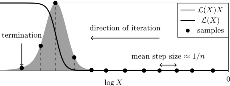
Figure 2.1: A schematic representation of nested sampling with a constant number of live points n. The curve L(X)X shows the relative posterior mass, the bulk of which is contained in some small fraction of the prior and is only visible on a log scale in

X. The algorithm iterates inwards inX exponentially with stochastic shrinkage ratios distributed according to (2.18).

some value_L∗ asX(_L∗), where

X(_L∗)_≡

Z

L(θ)>L∗

π(θ) dθ, (2.16)

and X ∈ [0,1]. Provided the inverse L(X) ≡ X−1(L) exists,3 the evidence (2.13) can be expressed as

Z=

Z 1 0 L

(X) dX. (2.17)

Given a set of dead points with likelihoods _Li, the corresponding prior volumes Xi are unknown but are modelled statistically as Xi = tiXi−1, where X0 = 1 and each

shrinkage ratioti is independently distributed as the largest ofnrandom variables from the interval [0,1] (Skilling, 2006). Hence:

P(ti) =ntni−1, E[logti] =− 1

n, Var[logti] =

1

n2, (2.18)

and the algorithm samples within an exponentially shrinking part of the prior. This exponential shrinkage is shown schematically in Figure 2.1.

3_{A sufficient condition for}

L(X) ≡ X−1(L) to exist is for L to be continuous and π to have a connected support. See Chopin and Robert (2010) and Feroz et al. (2013, Appendix C) for a more detailed measure-theoretic discussion.

(29)

Evidence estimation

Nested sampling therefore allows one to approximate the evidence (2.17) via a quadra-ture sum over the dead points

Z(t)_≈ X i∈dead

Liwi(t), (2.19)

where t = _{t1, t2, . . . , tndead} are the unknown set of shrinkage ratios for the ndead

iterations of the nested sampling process, and each ti is an independent random vari-able drawn from distribution (2.18). The shrinkage ratios define the prior volumes via

Xi(t) =Qik=0tk, and thewi are appropriately chosen quadrature weights roughly cor-responding to the volume of the “prior shell” to which a given dead point belongs. For example, using the trapezium rule: wi(t) = 1₂(Xi−1(t)−Xi+1(t)).4

Given that the shrinkage ratiostarea priori unknown, we may quantify our knowl-edge of_Z by simulating sets oftaccording to (2.18), and working with the distribution of the resulting set of evidences _{Z}_t from (2.19) (Skilling, 2006). Typically one then computes and reports a mean value and error for log_Z from this distribution.

Several alternative methods for calculating evidence inferences are reported in the literature. Skilling (2006) also proposes an error calculation based on relative entropy, which demonstrates that the uncertainty of logZis dominated by the Poisson variability in the number of steps required to reach the bulk of the posterior mass. Keeton (2011) uses distribution moments and running totals which are updated with each nested sam-pling step. This method has been extended by Handley et al. (2015b) to allow the splitting of multi-modal likelihoods into different clusters and the treatment of variable numbers of live points. For a more detailed discussion of the convergence properties of nested sampling evidences, see Chopin and Robert (2010).

Thus, the dominant sampling error in the evidence estimate (2.19) from perfect nested sampling is from statistical variation in the unknown volumes of the prior “shells”

wi(t) that each point represents. The error from approximating the integral forZ with a sum can be safely neglected unlessnis very small5(Skilling, 2006). There is also some

4_{For the final dead point, as} _X

ndead+1 is not available, wndead(t) can be approximated with wndead−1(t). The remaining prior volume after the final dead point can be ignored, or included in

calculations using the live points remaining at termination (a method for doing this is described in Section 5.2). The trapezium rule weight of the first point can be increased to assign it all prior volume betweenX = 1 andX=X1, but this typically makes negligible difference in practice.

5_{The trapezium rule error is}

O(1/n2_{), and if required other methods such as Simpson integration}

(30)

error from terminating the algorithm and truncating the sum, but this is can be made negligible with appropriate termination conditions.

Parameter estimation

One may also perform posterior inference from nested sampling by using the dead points to construct a set of posterior samples with weights proportional to their share of the posterior mass (Skilling, 2006):

pi(t) = wi(t)Li P iwi(t)Li = wi(t)Li Z(t) . (2.20)

As before,t is the set of prior shrinkage ratios and in the trapezium rule casewi(t) =

1

2(Xi−1(t)−Xi+1(t)). The resulting sampling errors are discussed in detail in Chapter 3. 2.4.2 Implementations

Significantly, the nested sampling algorithm as described above does not prescribe any specific method for generating samples from within iso-likelihood contours. Since nested sampling’s inception, a variety of techniques have been applied to this problem. Some popular methods are (Handley et al., 2015b):

• MCMC-based sampling, the method originally envisaged by Skilling, which re-quires taking a number of steps along the MCMC chain between successive samples used in the nested sampling run to ensure they are decorrelated. However, tradi-tional Metropolis-Hastings or Gibbs sampling requires a large amount of tuning of the proposal distribution to perform the required sampling efficiently (Feroz and Hobson, 2008). Two alternatives are Hamiltonian nested sampling (Betancourt, 2011) and Galilean nested sampling (Feroz and Skilling, 2013; Skilling, 2012), which use Hamiltonian Monte Carlo and Galilean Monte Carlo respectively. Both approaches have momentum-like auxiliary parameters and allow Markov chains to “bounce” off the hard likelihood constraint. However these approaches re-quire gradients and a careful choice of step size, and can become inefficient for iso-likelihood contours which are difficult to bounce back into due to their shape (Feroz and Hobson, 2008).

• Rejection sampling is used in the popular MultiNest software (Feroz and

(31)

method introduced by Mukherjee et al. (2006). This involves enclosing the iso-likelihood contour in multiple overlapping ellipsoids, which are calculated using the live points, then sampling randomly from within this volume. Samples which do not satisfy the likelihood constraint are discarded. This is highly effective in modest dimensions, but the acceptance rate decreases exponentially with dimen-sionality.

• Slice sampling (Neal, 2003) was applied to nested sampling by Aitken and Akman (2013) and is used by PolyChord (Handley et al., 2015a,b). At each iteration, a random live point and a random direction are selected. Points are sampled along the line (“chord”) with the chosen direction which intersects the chosen live point, in order to establish the bounds at which the line intersects the iso-likelihood contour. A point is then sampled along this line from within the contour. To prevent the new point from being correlated with the live point through which the chord passes, this process is repeated multiple times. While this is less ef-ficient than rejection sampling in low dimensions, it becomes more efef-ficient for high dimensional problems; computational costs withPolyChord scale as _O(D3₎

whereas for MultiNest they scale exponentially. For a more detailed description

of PolyChord’s sampling method, including a diagram illustrating the process, see

Handley et al. (2015b, Section 4).

Furthermore, a number of nested sampling variants have been proposed which al-ter the algorithm described in Section 2.4.1. Most notably, diffusive nested sampling (Brewer et al., 2011) uses a number of MCMC chains to sample a mixture of nested probability distributions. This approach is implemented in the DNestsoftware package

and has been applied to a number of astronomical problems (see for example Pancoast et al., 2014). In addition, superposition-enhanced nested sampling (Martiniani et al., 2014) combines nested sampling with global optimization techniques to improve the algorithm’s ability to find all the modes in highly multimodal spaces. Salomone et al. (2018) propose another hybrid approach involving Sequential Monte Carlo (mentioned in Section 2.3).

Having provided an overview of Bayesian inference and nested sampling methods in this chapter, we next present our work on estimating the uncertainty and reliability of nested sampling calculations in Chapters 3 and 4. This is followed in Chapter 5 by a

(32)

description of our dynamic nested sampling algorithm, which can greatly increase the computational efficiency of nested sampling calculations.

(33)

Chapter 3

Sampling errors in nested

sampling parameter estimation

This chapter provides the first explanation of the two main sources of sampling errors in nested sampling parameter estimation, and presents a new diagrammatic representation for the process. We find no previously existing method can accurately measure the parameter estimation errors of a single nested sampling run, and propose a method for doing so using a new algorithm for dividing nested sampling runs. The material presented is an edited version of Higson et al. (2018).

3.1 Introduction

Sampling errors in nested sampling parameter estimation differ from those in Bayesian evidence calculation, but have been little studied in the literature. As a result these errors are poorly understood compared to other numerical methods, despite the growing popularity of the technique and its widespread use in astronomy.

Correctly quantifying uncertainty due to sampling errors is vital for identifying spu-rious results. Conversely, finding such errors are very small may imply an unnecessarily large amount of computational resource is being used for the calculation. This chapter has two goals: to provide an explanation of the sources of these errors and an empir-ical technique for estimating them. One obvious method is to repeat the analysis a number of times, although this increases the computational cost by a corresponding factor. Interestingly, we find no current method can accurately estimate these errors

(34)

on parameter estimates from a single analysis, and so we present a new method for doing this. Our approach uses a new algorithm for dividing a single nested sampling run into multiple valid nested sampling runs; these can then be recombined in different combinations using resampling techniques such as the bootstrap. We test our results and new method empirically.

The chapter begins with background on sampling errors in parameter estimation from posterior samples. We then explain the two main sources of sampling errors in nested sampling parameter estimation in Section 3.3, and present a new diagrammatic representation of the process (illustrated in Figures 3.2a to 3.2e). Section 3.4 describes our new method for measuring sampling errors from a single nested sampling run, using our new algorithm for division of such runs.

We empirically test our method’s accuracy in Section 3.5 with the help of analytical cases in the manner described by Keeton (2011). Here one can obtain uncorrelated samples from the prior space within some likelihood contour using standard techniques, and we term the resulting procedureperfect nested sampling. Results in Section 3.5 were calculated using an early version of the perfectns software package (Higson, 2018c). In Section 3.6 we test sampling error estimates from our method for PolyChord calcu-lations, and Section 3.7 describes the application of these sampling error estimates to gravitational waves in Chua et al. (2018). Our approach accurately quantifies uncer-tainties on parameter estimates from the stochasticity of the nested sampling algorithm, but software used for practical problems may produce additional errors from correlated samples within likelihood contours that are specific to a given implementation — these are discussed in detail in Chapter 4. Our method gives superior performance to the current approach and can be easily be applied to existing nested sampling software; we have implemented it in thenestcheck software package (Higson, 2018b).

3.2 Background: sampling errors in parameter

estimation

Sampling techniques such as nested sampling provide information about a posterior distribution_P(θ) by producing a set of weighted samples

(35)

where each θs is drawn from P(θ) with probability proportional to ps× P(θs), and

P

s∈Sps = 1. Numerical results are then computed from the samples S. For example, the posterior expectation of a function of the parametersf(θ) can be estimated as

E[f(θ)] =

Z

f(θ)_P(θ)dθ _≈ X

s∈S

psf(θs). (3.2)

In this case the sampling error is the difference between P

s∈Spsf(θs) and the exact value of E[f(θ)]. Often the posterior distributions of parameters θ are of interest, and are estimated numerically from the samples by dividing the parameter space into cells or via kernel density estimation.

There have been many works on approximating MCMC sampling errors, including investigation of quantiles and the amount of computation required to reach some level of accuracy — see for example Doss et al. (2015), Flegal et al. (2008) and Liu et al. (2016). In particular Sequential Monte Carlo samplers (mentioned in Section 2.3) have similarities with nested sampling, and their sampling errors are better understood. For some related methods such as the Tootsie Pop algorithm (Huber and Schott, 2014) and accelerated simulated annealing (Bez´akov´a et al., 2008) the error distribution is known exactly, although these techniques are less widely used. This chapter introduces empirically tested techniques for quantifying sampling errors from the nested sampling algorithm.

In nested sampling parameter estimation, the sample weights (2.20) present a de-parture from traditional sampling approaches in that the wi(t) are random variables, with their stochasticity determined by (2.18). When computing expectations (3.2) there is now an additional error associated with our lack of knowledge of the precise values

pi(t). Nested sampling software packages such as MultiNest and PolyChord produce posterior files containing only the expected values

E[pi(t)] = e−i/n_L i P je−j/nLj . (3.3)

To account for the stochasticity in the weightspi, Skilling (2006) suggests simulating the prior volume shrinkage ratios t in the same manner as for evidence estimation (mentioned in Section 2.4.1), and using these simulations to calculate a set of values for estimators such as (3.2). The sampling error should then be estimated from the variation within this sample; we term this the simulated weights method. We believe

(36)

this procedure is the only estimate of sampling errors in parameter estimation from a single nested sampling run proposed in the literature. However it is in general an

underestimate, as can be seen in the numerical tests in Section 3.5. Appendix 3.B discusses this underestimation of errors in detail.

We now describe why the simulated weights method does not capture all sources of sampling errors, and in Section 3.4 we propose a new method for correctly computing these errors.

3.3 Sources of sampling errors in nested sampling

parameter estimation

In order to understand why the simulated weights method underestimates sampling errors, we require a result from Chopin and Robert (2010). They show that the expec-tation integral (3.2) may be re-phrased in terms of the prior volume X via:

E[f(θ)] = Z f(θ)_P(θ)dθ= Z f(θ)L(θ)π(θ) Z dθ= 1 Z Z ˜ f(X)_L(X) dX, (3.4)

where ˜f(X) is the prior expectation off(θ) on some iso-likelihood contourL(θ) =L(X), ˜

f(X)_≡Eπ[f(θ)_|L(θ) =_L(X)]. (3.5)

The simulated weights approach amounts to discretising the integral (3.4) as 1 Z Z ˜ f(X)L(X) dX≈ 1 Z X i ˜ f(Xi)Li 1 2(Xi−1−Xi+1), (3.6) and, most importantly, further requiring that we may use f(θi) as a proxy for ˜f(Xi) at each point Xi. In some special cases f(θi) = ˜f(Xi) for all θ and this approach is valid, for example whenf(θi) = ˜f(Xi)∝ −logLi(entropy computation), but in general it is not. This can cause significant inaccuracies as iso-likelihood contours often span wide ranges of different parameter values, as illustrated in Figure 3.1 (based on Figure 1 in Handley et al., 2015a). There are also some errors from discretising the integral in (3.6) using the trapezium rule, but these are typically small unless the number of live pointsnis low. Furthermore, errors due to the truncation of the sum in (3.6) when the algorithm terminates can be made negligible with appropriate termination conditions.

To summarise, the dominant sampling errors in estimating some parameter or func-tion of parameters from perfect nested sampling typically come from two sources:

(37)

θ₂ θ₁ 5 4 3 2 1

Figure 3.1: Nested sampling dead points and iso-likelihood contours for a two-dimensional multi-modal likelihood_L(θ); darker shading shows higher likelihoods. Iso-likelihood contours can pass through a wide range of different parameter values.

(i) approximating the unknown prior volumes wi(t) with their expectation E[wi(t)] using (2.18);

(ii) approximating the mean value of a function of parameters over an entire iso-likelihood contour ˜f(Xi) with its value at a single pointf(θi).

Errors from (i) are also present in evidence calculation; in the parameter estimation case they are typically smaller as results depend only on the relative weights of the samples. In contrast (ii) is only present in parameter estimation, where it is typically a significant or dominant source of sampling errors. The relative contributions of (i) and (ii) are empirically tested in Appendix 3.A, where they are calculated for analytical cases by using exact values for weights wi(t) and by replacing f(θi) with ˜f(Xi). The simulated weights method underestimates sampling errors in parameter estimation as it ignores errors from (ii).

We now introduce a new diagrammatic representation of nested sampling parameter estimation to illustrate the two different sources of sampling errors.

(38)

3.3.1 Diagrammatic representation

Nested sampling transforms evidence calculations of any dimension into a 1-dimensional problem1 _in _L₍_X_{) which can be entirely represented on a diagram like Figure 2.1. An}

analogous diagram for parameter estimation must also illustrate sampling a single point

f(θi) on each iso-likelihood contourL(θ) =L(Xi) from the distribution P(f(θ)|Xi). We propose a generalisation of Figure 2.1 for visualising parameter estimation prob-lems, and present it in Figures 3.2a to 3.2e. The top panel in each figure is similar to Figure 2.1 and shows the relative posterior mass L(X)X at each value of logX. The lower central panel shows the probability distribution P(f(θ)|X) and its mean ˜f(X). The posterior distribution is shown on the left — this is equal to the distributions

P(f(θ)|X) (the lower central panel) marginalised overX in proportion to the posterior weight at each X (the top panel).

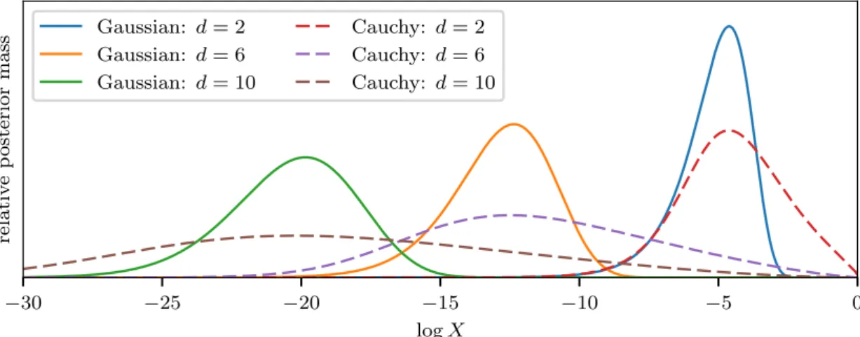
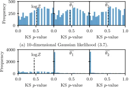
For these example plots we use d-dimensional spherical unit Gaussian likelihoods

L(θ) = (2π)−d/2e−|θ|2/2 _(3.7)

and d-dimensional spherical unit Cauchy likelihoods

L(θ) = Γ( 1+d 2 ) π(d+1)/2 1 +_|θ_|2 −(d+1₂ ) , (3.8)

withd-dimensional co-centred spherical Gaussian priors

π(θ) = (2πσ_π2)−d/2e−|θ|2/2σ2π_. _(3.9)

Here Γ denotes the gamma function, and in this chapter all Gaussian priors (3.9) use

σπ = 10. We denote the first component of the θ vector as θˆ₁, although by symmetry

the results will be the same for any component. θˆ₁ and θ_ˆ₁2 are the first and second

moments of the posterior distribution ofθˆ₁.

The form of the distribution P(f(θ)|X) as X varies depends on the likelihood only through the shape of the iso-likelihood contours L(θ) = L(X). Therefore the lower central panel of the diagrams for some f(θ) is the same for any likelihoods with the same contours — this can be seen in Figures 3.2a and 3.2b, where the differences in

1_{For practical nested sampling problems implementation-specific errors can differ for two likelihoods}

with the same L(X). For example if one likelihood has a much higher dimension and a much larger number of modes than the other, it may have larger errors from the software failing to explore the parameter space fully.

(39)

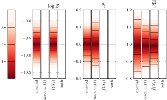
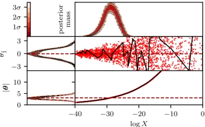
relative posterior mass −16 ₋14 ₋12 ₋10 ₋8 ₋6 ₋4 ₋2 0 logX ˜ f(X) E[f(θ)_|L, π] posterior −10 −5 0 5 10 f ( θ ) = θˆ 1 1σ 2σ 3σ

(a) f(θ) =θˆ1 with a 5-dimensional Gaussian likelihood (3.7) and a Gaussian prior (3.9). relative posterior mass

−16 ₋14 ₋12 ₋10 ₋8 ₋6 ₋4 ₋2 0 logX ˜ f(X) E[f(θ)_|L, π] posterior −10 −5 0 5 10 f ( θ ) = θˆ 1 1σ 2σ 3σ

(b)f(θ) =θˆ1with a 5-dimensional Cauchy likelihood (3.8) and a Gaussian prior (3.9). relative posterior mass

−16 −14 −12 −10 −8 −6 −4 −2 0 logX ˜ f(X) E[f(θ)|L, π] posterior −10 −5 0 5 10 f ( θ ) = θˆ 1 1σ 2σ 3σ

(40)

relative posterior mass −16 ₋14 ₋12 ₋10 ₋8 ₋6 ₋4 ₋2 0 logX ˜ f(X) E[f(θ)_|L, π] posterior 0 2 4 6 8 10 f ( θ ) = θ 2 ˆ 1 1σ 2σ 3σ (d)f(θ) =θˆ1

2_{with a 5-dimensional Gaussian likelihood (3.7) and a Gaussian prior (3.9).}

relative posterior mass

−16 ₋14 ₋12 ₋10 ₋8 ₋6 ₋4 ₋2 0 logX ˜ f(X) E[f(θ)_|L, π] posterior 0 2 4 6 8 10 f ( θ ) = | θ | 1σ 2σ 3σ

(e) f(θ) = _|θ_| (i.e. the radial distance from the likelihood’s maximum) with a 5-dimensional Gaussian likelihood (3.7) and a Gaussian prior (3.9). In this case f(θi) = ˜f(Xi) for allθ and

sampling errors are only from uncertainty in prior volume shrinkages and the trapezium rule approximation.

Figure 3.2: Nested sampling parameter estimation diagrams: in each case the top panel shows the relative posterior mass at each value of logX (_{∝ L}(X)X). The lower central panel shows the distribution P(f(θ)_|X) of values f(θ) on each iso-likelihood contour L(θ) = L(X); the dashed line shows the expectation of this distribution which we defined in (3.5) as ˜f(X). The left panel shows the posterior distribution of f(θ), with the dotted line showing its posterior expectation. The colour scale shows the fraction of the cumulative probability distribution lying between some region and the median.

(41)

the posterior (left panel) are due only to the different posterior weights in logX (top panel). Adapted versions of these diagrams which can be easily made from the samples produced by nested sampling software fora priori unknown likelihoods are introduced in Chapter 4.

3.3.2 Transforming a parameter estimation problem into 2 dimensions

As illustrated by our diagrams, nested sampling parameter estimation is fundamentally a 2-dimensional problem inL(X) andP(f(θ)|X). In fact a perfect nested sampling pa-rameter estimation calculation for somef(θ) givenL(θ) is equivalent to a 2-dimensional problem for f∗(θ∗) givenL∗₍_θ∗_{) when}

L∗(θ∗) =L(X), (3.10)

P(f∗(θ∗)_|X) =P(f(θ)_|X), (3.11) for all X. Any transformation satisfying (3.10) and (3.11) will leave our proposed diagram for the calculation unchanged. Parameter estimation can also be represented as a 1-dimensional problem in L∗₍_θ∗_{) =} _L₍_X_{) combined with a univariate stochastic}

process for each dead point iwith the distributionP(f(θ)|Xi).

One way to express a general nested sampling calculation in 2 dimensions is to map it onto the unit square θ∗ = (X, Y) with uniform priors X, Y ∈[0,1] and a likelihood L∗₍_θ∗_{) =} _L₍_X_{) which is independent of} _Y _{and satisfies (3.10). In this case} _X _{is, as}

before, the remaining fractional prior volume and Y parameterises each iso-likelihood contour. Using inverse transform sampling, for a general f(θ) a corresponding f∗(θ∗) satisfying (3.11) is

f∗(θ∗) =f∗(X, Y) =F−1(Y|X), (3.12) whereF−1(Y_|X) is the inverse of the cumulative distribution

F(Y_|X) =

Z Y

−∞

P(f(θ) =h_|X) dh. (3.13)

As an example let us considerd-dimensional spherically symmetric likelihoods such as (3.7) or (3.8) with co-centred spherically symmetric priors such as (3.9). ThenX(θ) is a function only of the radial distance from the centre_|θ_|, and the iso-likelihood contours L(θ) =_L(X) are hyperspherical shells of some radius_|θ_|_X. The probability distribution

(42)

of a single parameter θˆ1 (a single component ofθ) on such an iso-likelihood contour is then P(θˆ₁|X) =        Γ(d 2) |θ|XΓ(12) Γ( d−1 2 ) 1₋ θ 2 ˆ 1 |θ|2X d−₂3 if _{− |}θ_|_X < θˆ₁ <|θ|X, 0 otherwise. (3.14)

θˆ1 can be sampled directly or used to calculate the inverse cumulative distribution

which together with knowledge of the function_L(X) allows the parameter estimation of a d-dimensional Gaussian to be transformed into a 2-dimensional problem on the unit square.

Samples from (3.14) can be generated efficiently using the symmetry around θˆ₁ = 0

and the change of variables Θ =θ2_ˆ₁/|θ_|2_X to give a Beta distribution

P(Θ|X) =      Γ(d 2) Γ(1₂)Γ(d−₂1)Θ −12(1−Θ) d−3 2 if 0<Θ<1, 0 otherwise, (3.15) Θ∼Beta 1 2, d−1 2 . (3.16)

This technique is used for the numerical tests in Section 3.5 withperfectns, and allows

the efficient sampling of high dimensional spherically symmetric distributions where only a few parameters are of interest without generating all the remaining uninteresting parameters.

3.4 Estimating sampling errors in nested sampling

parameter estimation

Following the discussion of sources of sampling errors in Section 3.3, we seek a method for correctly calculating parameter estimation sampling errors from a single nested sampling run. As no additional samples θi are available, a natural starting point is to utilise resampling techniques such as the jackknife (Tukey, 1958), bootstrap (Efron, 1979) and Bayesian bootstrap (Rubin, 1981), which estimate the uncertainty on inferences from a set of samples by calculating the variation when samples are re-weighted.

However, as described in Section 2.4.1, the uncertainty in nested sampling weights

(43)

process. These are not accounted for by na¨ıvely applying jackknives and bootstraps to posterior samples produced by nested sampling, and these approaches fail when tested numerically. We instead require a method for dividing runs in a manner that preserves the statistical properties of nested sampling. No such method exists in the literature, so we present one in the remainder of this section.

3.4.1 Dividing runs into threads

Skilling (2006) describes how several nested sampling runs r = 1,2, . . . with n(r) _live

points may be combined simply by merging the dead points and sorting by likelihood value. The combined sequence of dead points is equivalent to a single nested sampling run withn=P

rn(r) live points.

In fact, as we show now, the reverse procedure is also possible. A nested sampling run with n points can be unwoven into a set of n valid nested sampling runs, each with n(r) _{= 1. We term these single live point runs} _threads_{. During nested sampling,}

each dead pointiis replaced by a new point sampled uniformly within its iso-likelihood contour_L(θ) =_Li. Starting from each initial live point that is generated, one may follow this sequence of replacements down the set of dead points. This sub-sequence of dead points is in fact a nested sampling run withn= 1. Our algorithm for dividing a nested sampling run into its constituent threads is presented more formally in Algorithm 2.

Result: nthreads.

Data: Dead points and the iterations at which they were sampled for a nested sampling run withn live points.

Rank dead points by likelihood in ascending order;

while i_∈ndo

make a new stack i;

select one of the initial points sampled at the start of the run; move the point out to the stack i;

while iteration < final iteration do

select point sampled at the iteration where previous point was replaced (“died”);

move the point to the stacki;

end end

Algorithm 2:Splitting a nested sampling run into threads.

(44)

1. splitting a run by randomly selecting some fraction of the dead points will not produce threads (i.e. single point nested sampling runs);

2. one may split a given nested sampling run into separate runs withn(r)₆= 1 by first separating into threads, and then recombining threads as desired;

3. the algorithm can be easily adapted for varying numbers of live points by permit-ting it to select multiple points on contours where n increases. This can result in constituent threads stopping or dividing into multiple threads part of the way through the run;

4. typically there is only one point which was sampled uniformly from the prior volume within each dead point i’s iso-likelihood contour _L(θ) = _Li — the point which replaced i. A sufficient condition for a nested sampling run to only have one unique division into threads is that_L(X) is an injective function;

5. in order for the threads to be true nested sampling runs, care must be taken with the termination conditions conditions used. See Appendix 3.D for a full discussion.

Given that threads represent independent nested sampling runs, one may apply stan-dard resampling techniques to the set of threads and approximate the entire sampling error distribution without making assumptions about its form. This works as the logXi values of the dead pointsifrom some run withnlive points form a Poisson process with rate n, meaning the logXj values of the dead points j of a single thread are a Poisson process of rate 1. For typical problems with computationally expensive likelihoods the computational cost of even a large number of resampling replications is negligible.

Having introduced a framework for applying resampling to nested sampling param-eter estimation we now present an example method using bootstrap resampling.

3.4.2 Bootstrap estimate of sampling errors

Givennobservationsx= (x1, . . . , xn), the bootstrap (Efron, 1979) creates new data sets

x∗_b by drawing nsamples fromx with replacement. This corresponds to approximating the probability distribution of a single data point x as

P(x)_≈ 1 n n X i=1 δ(x₋xi), (3.17)